Random Gene Signatures 'Predict' Survival in TCGA, and the 'Optimal' Cut-Point Makes Nearly Half of Useless Markers Significant
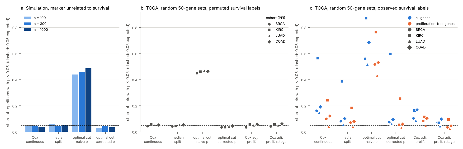
We scored 1,000 random 50-gene signatures against progression-free survival in four TCGA cohorts and simulated a marker with no link to survival. Picking the 'optimal' cut-point and reporting its log-rank p gave p < 0.05 for 44-49% of null markers. In kidney cancer, 57% of random signatures came out prognostic; with proliferation and stage in the model, that fell to 4-10% across the four cohorts.
The numbers here come from a simulation with a known answer and from public TCGA data. Scripts, outputs and the figure are public, and CI checks that the simulation and the scoring reproduce exactly. Before writing this up we downloaded the TCGA files again (same md5 sums) and re-ran everything on our own server with newer package versions (survival 3.7.0, maxstat 0.7.26). The p-value table came out byte-for-byte identical: 17,608 rows, 104,040 p-values. No client data is used. (한국어판: 무작위 유전자 세트도 생존을 «예측»한다)
A Kaplan-Meier plot with two curves pulling apart and "p = 0.003" in the corner is how a lot of prognostic biomarkers get introduced. We wanted to know how much that picture can be trusted when the split between "high" and "low" was chosen on the same data, and how often a gene signature looks prognostic when its genes were picked at random.
The short answer: choosing the "optimal" cut-point and printing the p-value of that split turned 44-49% of markers with no link to survival into significant ones. In TCGA kidney cancer, 57% of random 50-gene signatures were associated with progression-free survival in a plain Cox model. Adjusting for proliferation and stage removed most of that, though not all of it.
How the "optimal" split is usually made
library(survival); library(survminer)
cut <- surv_cutpoint(d, time = "time", event = "event", variables = "score")  # search for the best split
d2  <- surv_categorize(cut)
fit <- survfit(Surv(time, event) ~ score, data = d2)
ggsurvplot(fit, data = d2, pval = TRUE)   # prints the log-rank p of the chosen split
surv_cutpoint tries every split between the 10th and 90th percentile of the score and keeps the one with the largest standardised log-rank statistic. The plot then shows the p-value of that one split, computed as if nobody had looked at the others. You cannot tell from the figure that a search took place.
There is a second, older problem. Venet and colleagues showed in 2011 that most random gene sets are associated with breast cancer outcome, largely because so many genes move with proliferation. We checked whether that still holds in TCGA, and in cancers other than breast.
What we ran
For the simulation, the marker and the survival times were drawn independently: exponential survival, uniform censoring, about 37% of patients with an event. We used n = 100, 300 and 1,000, with 1,000 repetitions each. Two more settings with a real effect measure power, a linear one (hazard ratio 1.25 per SD) and a threshold one (HR 2 in the top quarter, 42% events).
For TCGA, expression came from UCSC Xena (gene-level RSEM, log2(normalised count + 1), 20,530 genes), with each gene z-scored within its cohort. Survival and stage came from the TCGA Pan-Cancer Clinical Data Resource (Liu et al. 2018). We used progression-free interval as the endpoint, because breast cancer has too few deaths within TCGA follow-up for overall survival to be useful. Primary tumours only:
| Cohort | Patients | PFI events |
|---|---|---|
| BRCA | 1,081 | 145 |
| KIRC | 529 | 159 |
| LUAD | 502 | 206 |
| COAD | 278 | 81 |
A signature's score is the mean z-score of its genes. We scored four kinds:
- 1,000 random 50-gene sets drawn from all expressed genes
- 1,000 random 50-gene sets drawn only from genes nearly uncorrelated with proliferation (|r| < 0.2)
- the 11-gene PAM50 proliferation signature (BIRC5, CCNB1, CDC20, NUF2, CEP55, NDC80, MKI67, PTTG1, RRM2, TYMS, UBE2C)
- the 50 genes most correlated with that proliferation score, the 11 excluded, as a stand-in for Venet's meta-PCNA
With the real survival labels there is no ground truth for any single signature. So every analysis was also run with time and event shuffled together across patients. Under those permuted labels nothing can be associated with survival, and every p < 0.05 is a false positive.
Each marker went through the same analyses:
| Analysis | What is reported |
|---|---|
| Cox, continuous score | Wald p of the score |
| Median split | log-rank p, high vs low at the median |
| Optimal cut-point, naive p | best split between the 10th and 90th percentile (the surv_cutpoint search), then its log-rank p as if fixed in advance |
| Optimal cut-point, corrected p | the same search, with the p-value of the maximally selected statistic (maxstat, Lausen and Schumacher 1992) |
| Cox, adjusted | score plus the proliferation score; then also AJCC stage, on patients with a known stage |
A marker that has nothing to do with survival
Share of 1,000 simulated repetitions with p < 0.05. Without any signal the target is 0.05.
| n | Cox continuous | Median split | Optimal cut, naive p | Optimal cut, corrected p |
|---|---|---|---|---|
| 100 | 0.044 | 0.060 | 0.439 | 0.032 |
| 300 | 0.048 | 0.044 | 0.457 | 0.044 |
| 1,000 | 0.040 | 0.052 | 0.486 | 0.036 |
The naive p creeps up with sample size, from 0.44 to 0.49, which fits the idea that a bigger sample gives the search more room. With 1,000 repetitions the standard error is about 1.6 points, so n = 100 and 300 are not really distinguishable.
The chosen split also exaggerates the effect. We report hazard ratios folded to be at least 1, so a split with no real effect still shows something above 1. On that scale a fixed median split under the null gave a median HR of 1.14 at n = 300; the optimal split gave 1.56. At n = 100 the two were 1.26 and 2.13.
The corrected p behaves: 3.2-4.4% under the null. It is not free. For a linear effect it had less power than the Cox model (0.47 against 0.65 at n = 300). When the effect really had a threshold, it did better (0.83 against 0.75).
TCGA with shuffled survival
With permuted labels, the random 50-gene sets drawn from all genes reached p < 0.05 in 3.5-6.2% of cases under every analysis except one. With the naive optimal cut-point it was 45-47% in all four cohorts. Real expression data behave like the simulation.
TCGA with the real survival data
Share of 1,000 random 50-gene sets (all genes) with p < 0.05:
| Cohort | Cox continuous | Median split | Optimal cut, naive p | Optimal cut, corrected p | Cox adj. proliferation | Cox adj. proliferation + stage |
|---|---|---|---|---|---|---|
| BRCA | 0.162 | 0.082 | 0.561 | 0.075 | 0.104 | 0.071 |
| KIRC | 0.565 | 0.388 | 0.872 | 0.597 | 0.165 | 0.070 |
| LUAD | 0.150 | 0.056 | 0.517 | 0.061 | 0.089 | 0.044 |
| COAD | 0.193 | 0.102 | 0.687 | 0.095 | 0.170 | 0.099 |
In kidney cancer, more than half of all random 50-gene sets are prognostic in a plain Cox model, and 87% by the naive optimal cut-point.
Sets drawn only from proliferation-independent genes were prognostic less often: 24% in KIRC (against 57%), 10% in BRCA, 4% in LUAD and 12% in COAD. The proliferation signature itself was strongly prognostic in KIRC (p = 4.4 × 10⁻¹⁷), less so in LUAD (0.0026) and BRCA (0.031), and not at all in COAD (0.49). In KIRC, the 50 genes most correlated with proliferation went from p = 1.8 × 10⁻¹⁵ to p = 0.26 once the proliferation score was in the model.
Colon cancer is the odd one. Its proliferation score is not prognostic, adjusting for it barely moved the random sets (19.3% to 17.0%), and most of the drop to 9.9% came from stage. Even then 9.9% is still about twice what the same analysis gives with shuffled labels (6.2%), so something else carries signal there. Stromal content is a known candidate in colon cancer; we did not test it.
What we take from it
The cut-point problem is the bigger one, because it is a statistical error rather than biology. It turned close to half of all useless markers into significant ones in every data set we tried, simulated or real.
Random signatures being prognostic, on the other hand, reflects real biology: proliferation and stage are strongly tied to outcome, and many genes follow them. That changes what a new signature has to show. In KIRC it is not enough to be associated with survival; more than half of all random gene sets are. A Kaplan-Meier plot with p = 0.01 does not say whether a signature beats that base rate.
What to do instead
Use the continuous score in a Cox model as the main test, and keep any split for the picture. If a data-driven cut-point is needed, report the p-value that accounts for the search rather than the p-value of the split it found:
library(survival); library(maxstat)
mt <- maxstat.test(Surv(time, event) ~ score, data = d, smethod = "LogRank",
                   pmethod = "Lau92", minprop = 0.1, maxprop = 0.9)
mt$estimate   # the chosen cut-point
mt$p.value    # the p-value that accounts for the search
Better still, fix the cut-point in one cohort and test it in another. Before calling a signature prognostic, score a few hundred random signatures of the same size on the same data and see where yours falls. And put the known prognostic factors (proliferation, stage, grade) in the model before claiming the signature adds anything.
Limits
This is four TCGA cohorts and one endpoint, progression-free interval. Overall survival or other cancer types will give other shares, although the direction of the cut-point bias does not depend on the data. We used one signature size (50 genes) and one way to score it (mean z-score). The stage-adjusted models use only patients with a known stage (for example 1,057 of 1,081 in BRCA and 268 of 278 in COAD). In BRCA, stage IV has 20 patients, and some adjusted Cox fits warn about a diverging stage coefficient; it does not affect the p-value of the score. The simulation uses exponential survival with uniform censoring, which is tidier than real follow-up.
Reproduce it
Everything is in sbmlab-benchmarks/random-signatures-tcga. bash download.sh fetches about 150 MB from UCSC Xena. The simulation takes under a minute, the TCGA part 6-7 minutes on one core (R 4.3.3 with survival, maxstat and data.table). Other Xena cohorts can be passed by name.
References
- Venet D, Dumont JE, Detours V. Most random gene expression signatures are significantly associated with breast cancer outcome. PLoS Comput Biol 2011;7(10):e1002240.
- Altman DG, Lausen B, Sauerbrei W, Schumacher M. Dangers of using "optimal" cutpoints in the evaluation of prognostic factors. J Natl Cancer Inst 1994;86(11):829-835.
- Lausen B, Schumacher M. Maximally selected rank statistics. Biometrics 1992;48(1):73-85.
- Liu J, et al. An integrated TCGA pan-cancer clinical data resource to drive high-quality survival outcome analytics. Cell 2018;173(2):400-416.
- Nielsen TO, et al. A comparison of PAM50 intrinsic subtyping with immunohistochemistry and clinical prognostic factors in tamoxifen-treated estrogen receptor-positive breast cancer. Clin Cancer Res 2010;16(21):5222-5232.
Related
Related
It Almost Worked: Four Ways a Multi-Omics Pipeline Nearly Reported a False Success
Aug 10 · 19 min read
BioinformaticsSingle-Cell Differential Expression Between Patients: Cell-Level Tests Flag Up to 24% of Genes When Nothing Differs. Pseudobulk vs FindMarkers on Real Donors
Nov 9 · 9 min read
BioinformaticsCorrect Batch Effects, Then Test? With an Unbalanced Design, ComBat Turns a 5% False-Positive Target into 29%
Nov 4 · 10 min read
BioinformaticsSTRING Enrichment and the Background Trap: 300 Random Proteins, About 100 'Significant' GO Terms
Oct 13 · 7 min read