Biomarker Discovery and Data Leakage: Shuffled Labels Still Scored AUC 0.75 on a Real CSF Proteome

Picture a biomarker study with a few hundred samples, a thousand or more proteins, and a reported AUC of 0.85. Whether that AUC means anything depends mostly on one detail of the analysis: when the proteins were chosen.

If the panel is picked using all samples and the classifier is cross-validated afterwards, the samples used to test the model already helped choose its features. That is data leakage, and it inflates AUC. How much? I ran the test on a real proteomics cohort, with the labels shuffled so that the correct AUC is known to be 0.5.

The Short Version

Shuffled labels (no real signal), 20 proteins chosen from 1,484, 50 different shuffles:

How the AUC was obtained	Mean AUC	Range
No validation (score on the training samples)	0.83	0.75–0.89
Proteins chosen on all samples, then 5-fold CV	0.73	0.59–0.84
"External" cohorts, but proteins chosen using them too	0.75	0.52–0.88
Proteins chosen inside each CV fold (proper)	0.51	0.39–0.63
Train on two studies, test on the third, untouched (proper)	0.48	0.32–0.67

The three leaky ways of working turned pure noise into AUCs that would pass review. With 100 proteins instead of 20, the training AUC on noise was 0.99.

With the real labels the proper pipeline still reached AUC 0.91 on the untouched study (expected, because AD here is defined from CSF tau, which the proteomics also measures; this is not a diagnostic result). Leakage barely changed that number. It mattered where you can least afford it: when there was no signal at all.

The Data

Bader et al. 2020, Molecular Systems Biology: cerebrospinal fluid (CSF) proteomics of 197 people from three studies at four collection sites (the paper pools Magdeburg and Kiel as one study), with Alzheimer's disease defined biochemically from CSF tau and amyloid-β (88 AD, 109 controls). I used the authors' processed table (Dataset EV3: log10 intensities of 1,484 protein groups, 18% of values missing) and their sample table (EV2).

Cohort	AD	Control
Berlin	33	50
Sweden	29	31
Magdeburg	26	12
Kiel	0	16

The Test

The classifier is deliberately ordinary: median imputation, standardisation, choose the k proteins with the largest ANOVA F statistic, logistic regression. scikit-learn 1.9.1, 5-fold stratified cross-validation.

• Leaky CV: choose the proteins once, using all 197 samples, then cross-validate the classifier on those proteins.
• Proper CV: the protein selection is a step in the pipeline, so it is refitted on the training part of each fold and never sees the test fold.
• External: train on the Berlin and Sweden studies (143 people), test on the Magdeburg/Kiel study (54). In the leaky version the proteins are chosen using all samples first.
• Shuffled labels: randomly permute AD/control across samples. Any AUC above 0.5 is then produced by the analysis, not by biology. Each setting was run with 50 different permutations.

Here is the core of it, runnable on the two supplementary files:

import numpy as np, pandas as pd
from sklearn.pipeline import make_pipeline
from sklearn.impute import SimpleImputer
from sklearn.preprocessing import StandardScaler
from sklearn.feature_selection import SelectKBest, f_classif
from sklearn.linear_model import LogisticRegression
from sklearn.model_selection import StratifiedKFold, cross_val_score

# Bader et al. 2020, Dataset EV3 (log10 intensities) and EV2 (sample information)
e = pd.read_excel("MSB-16-e9356-s005.xlsx", header=None)
X = e.iloc[2:, 3:].astype(float).T
X.index = e.iloc[1, 3:]; X.columns = e.iloc[2:, 0]          # UniProt accessions (unique)
info = pd.read_excel("MSB-16-e9356-s004.xlsx").set_index("sample name")
info = info[info["primary biochemical AD classification"].notna()]
X = X.loc[[s for s in X.index if s in info.index]]
y = (info.loc[X.index, "primary biochemical AD classification"] == "biochemical AD").astype(int).values

cv = StratifiedKFold(5, shuffle=True, random_state=0)
clf = make_pipeline(SimpleImputer(strategy="median"), StandardScaler(), LogisticRegression(max_iter=5000))
pipe = make_pipeline(SimpleImputer(strategy="median"), StandardScaler(),
                     SelectKBest(f_classif, k=20), LogisticRegression(max_iter=5000))
Xi = SimpleImputer(strategy="median").fit_transform(X)
rng = np.random.default_rng(0)

leaky, proper = [], []
for _ in range(20):
    y_null = rng.permutation(y)                          # shuffled labels: the honest answer is AUC 0.5

    # Leaky: pick the 20 "best" proteins using ALL samples, then cross-validate the classifier
    keep = SelectKBest(f_classif, k=20).fit(Xi, y_null).get_support()
    leaky.append(cross_val_score(clf, X.loc[:, keep], y_null, cv=cv, scoring="roc_auc").mean())

    # Proper: selection is a step of the pipeline, so it only ever sees the training folds
    proper.append(cross_val_score(pipe, X, y_null, cv=cv, scoring="roc_auc").mean())

print(X.shape, f"leaky AUC {np.mean(leaky):.2f} (max {max(leaky):.2f}) | proper AUC {np.mean(proper):.2f} (max {max(proper):.2f})")

Output (a few seconds on a desktop CPU; this block uses 20 shuffles and one fixed fold split, while the tables below use 50 shuffles with a new fold split each, hence the small differences):

(197, 1484) leaky AUC 0.72 (max 0.83) | proper AUC 0.50 (max 0.67)

The only difference between the two numbers is whether SelectKBest sits outside or inside the cross-validation. (The leaky arm selects on data imputed with medians from all samples; that imputation does not use the labels, so the leak is the selection.)

Results

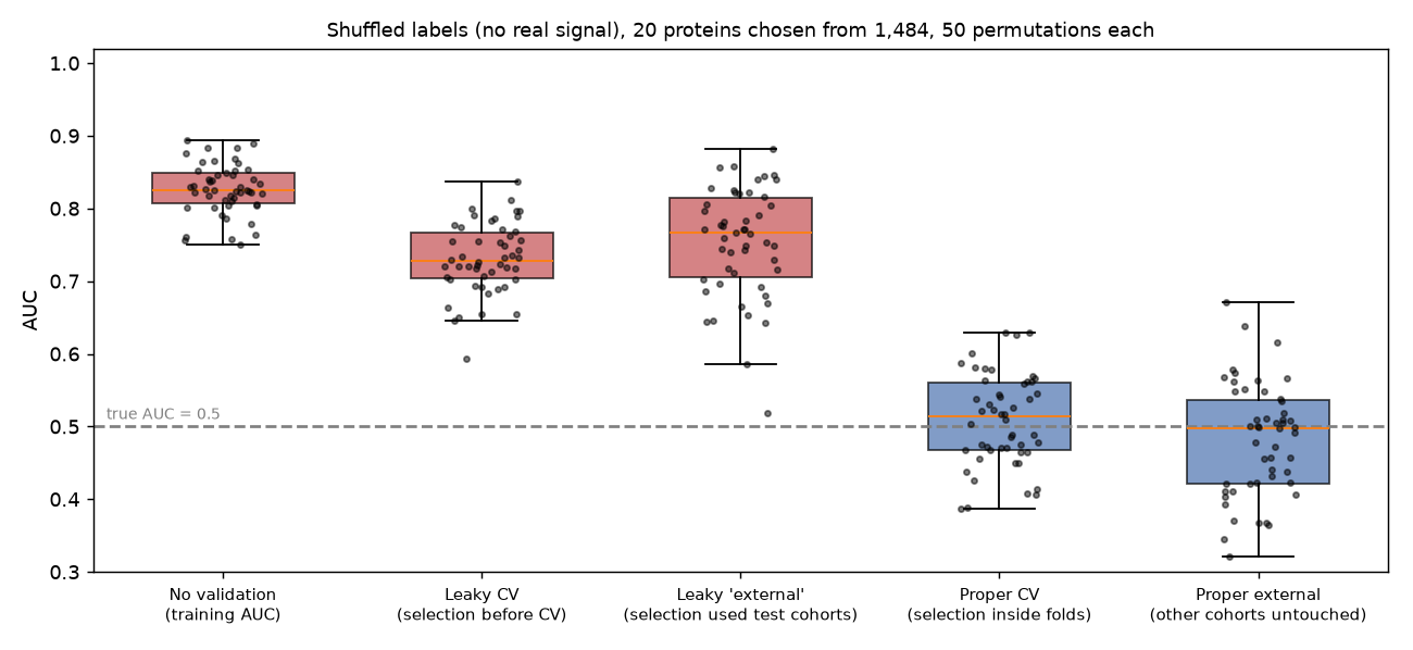Each dot is one shuffle of the labels. Red: leaky ways of estimating AUC. Blue: proper ones. The dashed line is the correct answer.

How many proteins you pick changes the illusion

Proteins chosen (shuffled labels, mean of 50)	No validation	Leaky CV	Proper CV
5	0.73	0.70	0.51
20	0.83	0.73	0.51
100	0.99	0.75	0.51

The more proteins the model uses, the better it fits noise, especially when nothing is held out. With 1,484 candidates and 197 samples, it is easy to find a set of proteins that lines up with an arbitrary labelling.

"External validation" does not help if the test cohorts chose the proteins

The most convincing-looking row is the leaky external one: the model was trained on the Berlin and Sweden studies and scored on the Magdeburg/Kiel study, which it never trained on. It still reached a mean AUC of 0.75 on shuffled labels, up to 0.88. The test samples had already voted on which proteins to use. An external cohort only counts as external if it played no part in any step, including protein selection, normalisation choices and the decision of which model to report.

With the real labels

Real labels, 20 proteins	AUC
No validation	0.95
Leaky CV (mean of 50 fold splits)	0.90
Proper CV (mean of 50 fold splits)	0.89
Leaky external (proteins chosen on all samples)	0.89
Proper external: Berlin + Sweden → Magdeburg/Kiel	0.91

Of the 20 proteins chosen on the training studies, 13 are in the paper's 40-protein panel (Dataset EV4), including tau (MAPT), SOD1, glycolytic enzymes (ALDOA, PKM, ENO2, LDHA), HPRT1, MIF and the 14-3-3 proteins YWHAG and YWHAZ. The other seven (FAM3C, NCAN, an SPP1 isoform group, GOT1, L1CAM, SMOC1, GDA) are not in the paper's panels. Here the signal is strong, and leakage added only about 0.01. In this test, leakage did not mainly inflate the real result; it manufactured results where there were none, and from the AUC alone you cannot tell which situation you are in.

Where Leakage Hides in Biomarker Pipelines

Feature selection is a common source, but not the only one (Kapoor & Narayanan 2023 give a taxonomy across 17 fields). Anything fitted on all samples before the split counts:

• choosing proteins by t-test, fold change, limma, LASSO or "top variable" on all samples;
• imputation, normalisation or batch correction fitted on all samples (usually smaller effects than selection, but real);
• tuning hyperparameters (k, λ, the model type) by the same cross-validation that is then reported;
• repeated measurements of the same person ending up on both sides of a split;
• trying several panels and reporting the best one, even if each was validated "properly".

For the label-dependent kinds (selection, tuning, picking the best panel) the check is the one used here: rerun the entire pipeline, every choice included, on many label shuffles. The mean AUC should sit at 0.5; one shuffle can land well above it by chance (in this test, proper pipelines reached 0.63 and 0.67 on single shuffles), so look at the average. This check does not catch steps that never use the labels, such as normalisation on all samples, or duplicate samples of one person: for duplicates, shuffle labels per person, not per sample.

What I Would Do

• Put every data-driven step inside the cross-validation: in scikit-learn, a Pipeline; in R, caret's sbf() or rfe(), or a tidymodels workflow whose recipe contains the selection step (supervised filters come from extension packages).
• If you also tune parameters, use nested cross-validation: tuning inside, performance estimate outside.
• Keep an external cohort sealed until the very end, and do not change the model after looking at it.
• Run the shuffled-label check over many shuffles and report it. It costs seconds.
• Report how the panel was chosen, not only the final AUC. For a reader, that sentence is worth more than the number.

Limits

• The real-label signal is partly circular. AD was defined from CSF tau and amyloid-β, and the proteomics measures tau (MAPT) itself, so a high real-label AUC is expected and is not a new diagnostic claim. The shuffled-label results do not depend on this.
• One dataset and one model. Other classifiers (random forests, SVMs) and other data sizes will give different numbers; the direction is the same in the published literature on selection bias (Ambroise & McLachlan 2002).
• Cohort composition. Kiel contributed only controls and Magdeburg mostly AD cases, so the external test mixes disease with site. With shuffled labels this cannot produce false signal (shuffling breaks it), but with real labels site effects could contribute.
• I used the authors' processed matrix, not a re-analysis of the raw files.

Related

• Biomarker discovery and validation: workflow and methods
• A MOGONET-style multi-omics biomarker pipeline
• Missing values in proteomics: six imputation methods scored

References

• Bader J.M. et al. (2020). Proteome profiling in cerebrospinal fluid reveals novel biomarkers of Alzheimer's disease. Molecular Systems Biology 16:e9356. doi:10.15252/msb.20199356 (data: Datasets EV2 and EV3; PRIDE PXD016278)
• Ambroise C., McLachlan G.J. (2002). Selection bias in gene extraction on the basis of microarray gene-expression data. PNAS 99:6562–6566. doi:10.1073/pnas.102102699
• Kapoor S., Narayanan A. (2023). Leakage and the reproducibility crisis in machine-learning-based science. Patterns 4:100804. doi:10.1016/j.patter.2023.100804