A MOGONET-Style Multi-Omics Biomarker Pipeline: Why a Near-Random Graph Net Still Earns Its Place

TL;DR (Quick Answer)

This is an honest engineering write-up of a MOGONET-style multi-omics consensus biomarker pipeline built as an internal R&D project at sysofti.

• The headline — on a small synthetic cohort (n=30), the graph network alone scores near-random in leak-free 5-fold cross-validation (AUC 0.53 ± 0.16). Yet as one voter in a 5-evidence consensus, the top-10 ranking is 90% real markers (9 of 10 are known periodontitis genes).
• The lesson — a single model that looks weak in honest evaluation can still be a useful voter. That contrast is the whole point of the consensus design, and we show it with data.
• What it is — per-omics Graph Convolutional Networks (GCN) over a sample-similarity graph, attention-fused, contributing to a consensus score alongside differential-expression hubs, Random Forest, a DNN, and co-expression modules.
• What it is not — the official MOGONET. We dropped the original's VCDN fusion for attention fusion. Call it "MOGONET-based." All numbers are from synthetic data with embedded ground-truth markers — code validation, not a clinical claim.

If you're implementing multi-omics integration, the parts you can't get from the paper are below: the real results, the leakage-aware evaluation, and the bugs we hit.

What MOGONET Is (the One-Line Mental Model)

MOGONET (Multi-Omics Graph cOnvolutional NETwork) learns a separate GCN per omics view on a sample-similarity graph (patients as nodes, edges by feature similarity), then fuses the per-view embeddings for classification and biomarker discovery. Reference: Wang et al. 2021, Nature Communications 12:3445; the GCN itself is Kipf & Welling 2017.

Mental model: "build one graph net per omics layer, let each form an opinion, then combine those opinions."

What We Simplified — and Why

The original MOGONET fuses views with a View Correlation Discovery Network (VCDN). We replaced it with attention-weighted fusion:

• Why — with tiny cohorts (tens of samples), VCDN's extra parameters were a liability; attention fusion gave a simpler intermediate-fusion scheme that still up-weights the more informative omics per sample.
• The tradeoff — we lose the explicit cross-view correlation modeling that is part of MOGONET's original contribution. So this is honestly MOGONET-based, not a reimplementation. The source docstring says as much: "Simplified implementation of MOGONET."

Architecture

Input: X_views = [omics1 (n×p1), omics2 (n×p2), ...]   (n = common samples)
  └─ per-view StandardScaler
  └─ per-view k-NN (cosine) adjacency  (n×n)
ViewEncoder (per omics):  GraphConv(p→128) → BN → ReLU → GraphConv(128→64)
  → view embedding (n×64)
Attention fusion:  softmax(Linear(64→1)) over views → weighted sum (n×64)
Classifier:  Linear(64→32) → ReLU → Linear(32→n_classes)

class GraphConvLayer(nn.Module):
    def __init__(self, in_features, out_features):
        super().__init__()
        self.linear = nn.Linear(in_features, out_features)
    def forward(self, x, adj):
        return torch.mm(adj, self.linear(x))   # propagate over the sample graph

class MOGONET(nn.Module):
    def __init__(self, input_dims, hidden_dim=128, latent_dim=64, n_classes=2):
        super().__init__()
        self.encoders = nn.ModuleList([ViewEncoder(d, hidden_dim, latent_dim) for d in input_dims])
        self.attention = nn.Linear(latent_dim, 1)
        self.classifier = nn.Sequential(nn.Linear(latent_dim, 32), nn.ReLU(), nn.Linear(32, n_classes))
    def forward(self, views, adjs):
        embeddings = [enc(x, adj) for enc, x, adj in zip(self.encoders, views, adjs)]
        stacked = torch.stack(embeddings, dim=0)                       # n_views × n × latent
        attn = F.softmax(self.attention(stacked).squeeze(-1), dim=0)   # per-view, per-sample
        fused = (stacked * attn.unsqueeze(-1)).sum(dim=0)              # n × latent
        return self.classifier(fused)

Sample-similarity graph — k-NN (cosine), no self-loops on purpose (see below):

def build_adjacency(X, k=5):
    sim = cosine_similarity(X)
    adj = np.zeros_like(sim)
    for i in range(len(sim)):
        top_k = np.argsort(sim[i])[-k-1:-1]      # top-k neighbours, excluding self
        adj[i, top_k] = sim[i, top_k]
        adj[top_k, i] = sim[top_k, i]            # symmetrize
    row_sum = adj.sum(axis=1, keepdims=True); row_sum[row_sum == 0] = 1   # guard zero-sum rows
    return adj / row_sum

The Engineering Decisions That Mattered

• Sample-node graph, not feature graph. Nodes are patients; edges are patient-patient similarity. Same-group patients cluster, so the GCN smooths group signal.
• No self-loops — on purpose. Standard GCN uses Ahat = A + I so a node keeps its own features. We deliberately omit the self-loop so each node's representation is built purely from its sample-neighborhood, pushing the model toward group structure rather than individual raw features. It is a tradeoff (you give up the node's own signal each layer), and we flag it as a choice, not an accident.
• Per-view scaling + common-sample intersection. Each omics standardized independently; only samples present in all views are used.
• Consensus over a single model. MOGONET is one of five evidence sources by design — Hub (DE+PPI), ML (Random Forest), DL (DNN), WGCNA co-expression, and MOGONET — with a multi-evidence bonus:

avg_score = sum(scores.values()) / max(len(scores), 1)
composite = avg_score * (1 + 0.3 * (n_sources - 1))   # reward agreement across sources

As the results show, this design choice is what makes the pipeline useful despite any single model being weak.

Results (Synthetic Data, with Ground Truth)

We validate on a synthetic periodontitis case-control set (3 omics — transcriptomics 500, proteomics 200, metabolomics 100 features × 30 samples, 15 disease / 15 control, seed-fixed) with known biomarkers deliberately embedded: up-regulated inflammatory genes (MMP8, MMP9, IL1B, IL6, TNF, RANKL, CTSK, TLR4 …) and down-regulated bone-formation genes (COL1A1, RUNX2, SP7, BGLAP, OPG …). Embedding known markers gives ground truth — you can check whether the pipeline recovers them, which is impossible on a real cohort.

Note on sources: the pipeline defines five evidence sources, but in this run WGCNA returned no co-expression hubs, so four sources actually contributed (Hub, ML, DL, MOGONET).

The consensus ranking surfaces real markers

Of 793 candidate features, the top-30 consensus included 13 of the 25 embedded markers. The ranking is strikingly clean at the top:

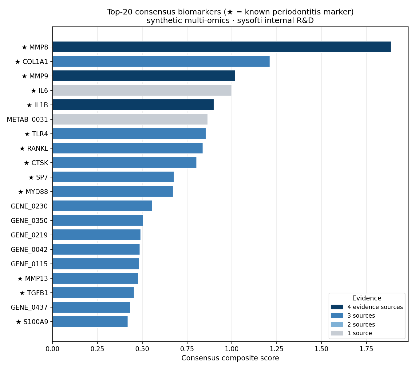
Rank	Gene	Composite	Sources	Known marker
1	MMP8	1.888	4	★
2	COL1A1	1.212	3	★
3	MMP9	1.020	4	★
4	IL6	1.000	1	★
5	IL1B	0.900	4	★
6	METAB_0031	0.866	1	—
7	TLR4	0.856	3	★
8	RANKL	0.838	3	★
9	CTSK	0.803	3	★
10	SP7	0.678	3	★
11	MYD88	0.672	3	★

• Precision@10 = 0.90 — 9 of the top 10 are known markers (only METAB_0031 is not).
• Recall@10 = 0.36, Recall@20 = 0.52 (9 then 13 of 25 known markers); it plateaus by 20 because a few embedded markers were given weak synthetic signal (e.g. TNF, fold-change ≈ 1.1).

More evidence = more trustworthy

Breaking the top-30 down by which sources agreed makes the consensus logic concrete:

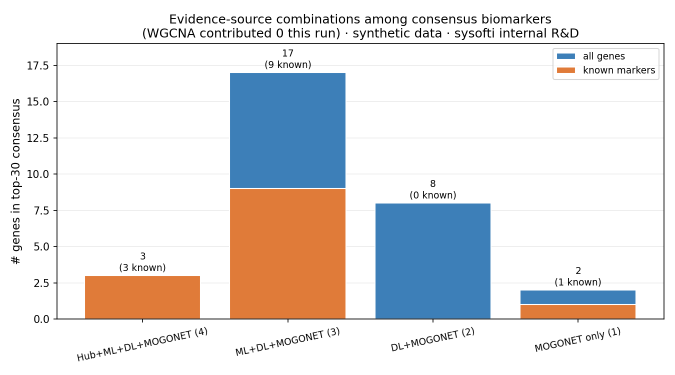
• 4 sources → 3 genes, all 3 known (100%): MMP8, MMP9, IL1B.
• 3 sources → 17 genes, 9 known.
• 2 sources (DL + MOGONET) → 8 genes, 0 known — pure noise.
• 1 source → 2 genes, 1 known.

The signal lives where independent methods agree. A gene flagged by four sources was always real here; genes flagged by only two were not.

The honest part: the graph net alone is near-random

We cross-validated MOGONET as a standalone classifier, rebuilding the sample graph from training folds only to avoid leakage:

MOGONET 5-fold CV AUC = 0.53 ± 0.16 (folds: 0.44, 0.44, 0.78, 0.33, 0.67)

That is barely above chance. With n=30 (six test samples per fold) and a transductive sample-graph model, a single GCN simply cannot generalize here — and its training AUC near 1.0 is mostly the leakage and the injected signal talking. This is exactly why MOGONET is wired in as one voter, not the decision-maker. The consensus result above is strong because it doesn't trust any single model, including this one.

Honest Limitations

1. Simplified model. No VCDN fusion — attention instead. "MOGONET-based," not a reimplementation.
2. MOGONET is a weak standalone classifier here (CV AUC 0.53). Useful only in aggregate. It also scores all 793 features, so its solo discriminative power is low.
3. Synthetic, small (n=30). Results validate the code's ability to recover injected signal — not clinical performance. External cohorts are required for any real claim.
4. Single run (seed 42). Known markers are stable at the top; the unnamed GENE_xxxx candidates shuffle on re-runs.
5. Self-loop omission is a design choice with a cost — worth A/B testing against the standard A + I formulation.
6. Feature importance is an approximation (first-layer weight magnitude), not a gradient-based attribution.

What Broke Along the Way (Real Notes)

• Zero-sum adjacency → NaN. If a sample's k-NN cosine similarities summed to zero, row-normalization divided by zero and propagated NaNs. Fixed with a row_sum[row_sum == 0] = 1 guard.
• Attribute-name mismatches (fixed twice). Pulling feature importance broke on AttributeError when the sklearn-wrapper conventions clashed with the nn.Module attribute names (view_encoders → encoders, model → model_).
• Common-sample collapse. When omics measured different sample sets, the intersection shrank fast. Added a "≥6 common samples" guard that skips gracefully instead of crashing.
• MOGONET scores everything. It assigns weight to all 793 features, so it appeared in all top-30 entries — the multi-evidence bonus is what keeps it honest.

What We'd Improve Next

• Report consensus performance under the same leak-free CV, not just MOGONET's.
• A/B test self-loops (Ahat = A + I).
• Gradient-based attribution (Integrated Gradients) instead of first-layer weights.
• Add VCDN fusion and compare head-to-head with attention fusion.
• External multi-omics cohort for real-world validation.

FAQ

Q: Is this the official MOGONET implementation?

No — a simplified, MOGONET-based design: per-omics GCN with attention fusion, without the original's VCDN view-correlation network.

Q: If MOGONET's CV AUC is only 0.53, why keep it?

Because it is one voter in a five-source consensus, not the classifier. Single models overfit small cohorts; consensus rewards agreement across independent methods, and that ranking recovered known markers at 90% precision in the top 10. A weak voter still adds signal when combined.

Q: Why validate on synthetic data?

Embedded known markers give ground truth, so you can measure recovery (recall/precision) — impossible on a real cohort where the answer is unknown. It validates the code, not clinical utility.

Q: Why omit GCN self-loops?

Intentional: without a self-loop, each node's representation comes purely from its sample-neighborhood, pushing the model toward group structure rather than individual features. It is a tradeoff worth A/B testing, not a universal recommendation.

Q: Can I use this on my own multi-omics data?

Yes — the classifier is sklearn-compatible (fit/predict/predict_proba). Build the sample graph from training data only to avoid leakage, and don't over-read AUC on small cohorts.

Resources

• Reference implementation (clean, standalone, MIT): github.com/shoo99/mogonet_lite
• Original paper: Wang T. et al. (2021), MOGONET integrates multi-omics data via graph convolutional networks for biomarker discovery, Nat Commun 12:3445.