DIA-NN 2.3 on a Known-Answer Benchmark: How It Compares With MaxQuant and FragPipe (and Why the Comparison Has a Catch)

This is the third post in a series where I run proteomics software myself on public data with a known answer and score every protein. The first two were MaxQuant 2.8 and FragPipe vs MaxQuant. This one adds DIA-NN.

The catch, up front: the benchmark dataset has DDA runs on an Orbitrap but no DIA runs on that Orbitrap. The DIA runs I used were acquired on a SCIEX TripleTOF 6600. So the comparison below mixes two things at once: the acquisition method (DIA vs DDA) together with the instrument, and the software. It tells you what each complete workflow produced on this sample, not which program is better.

The Short Version

Same samples (three per condition), same FASTA, 1% FDR, MaxLFQ-type protein quantities, match-between-runs on in all three:

	MaxQuant 2.8.1	FragPipe 24	DIA-NN 2.3.2
Acquisition	Orbitrap DDA	Orbitrap DDA	TripleTOF 6600 SWATH (DIA)
Proteins quantified, human / yeast / E. coli	2,896 / 907 / 132	4,605 / 1,817 / 359	5,477 / 2,374 / 446
All quantified, within ±0.5 of truth	98.8% / 92.3% / 81.1%	94.7% / 88.3% / 73.5%	98.6% / 95.1% / 85.4%
Same 3,866 proteins, within ±0.5	98.9% / 92.4% / 80.9%	99.7% / 99.3% / 97.7%	100% / 99.4% / 97.7%
Spread of human ratios (IQR, same 3,866)	0.14	0.14	0.04
Wall time	62 min	9 min	6 h 17 min (about 3.5 h of it reading .wiff files)

DIA-NN on the SWATH runs quantified the most proteins and produced by far the tightest ratios. On the proteins all three quantified, FragPipe and DIA-NN were equally often within ±0.5 of the truth; DIA-NN's ratios were about three times less spread out. Like FragPipe, the extra proteins only DIA-NN quantified were its least reliable part.

The Data

PRIDE PXD028735 (Van Puyvelde et al., Scientific Data 2022) mixes human, yeast and E. coli digests at known proportions:

	Human	Yeast	E. coli
Condition A	65%	30%	5%
Condition B	65%	15%	20%
Expected log2(B/A)	0	−1	+2

The same samples were measured on many instruments. For the DDA posts I used the Orbitrap Q Exactive HF-X runs. The dataset's Orbitrap files are DDA, AIF and gas-phase fractionation; there is no windowed Orbitrap DIA. The closest DIA option was TripleTOF 6600 SWATH, so I took the same design: Condition A and B, preparation batches Alpha, Beta and Gamma, first injection each (six runs, 30.3 GB).

Getting the files took longer than the analysis. PRIDE served about 27 KB/s per connection, and after a while refused new connections for long stretches. I split each file into ten ranged downloads; five of the six large .wiff.scan files still hit my retry limit and had to be resumed. About eight hours in total.

Settings and Commands

DIA-NN 2.3.2 for Windows, run from WSL on an i9-14900K with 64 GB RAM. SCIEX .wiff files need the Windows build; the Linux build cannot read them.

	MaxQuant / FragPipe (DDA posts)	DIA-NN (this post)
FASTA	Swiss-Prot human + yeast + E. coli (31,695 entries)	same file
Enzyme	trypsin, 2 missed cleavages	trypsin, 1 missed cleavage
Modifications	fixed carbamidomethyl C; variable oxidation M, acetyl protein N-term	fixed carbamidomethyl C; variable oxidation M (max 1)
Library	none (DDA search)	predicted from the FASTA (library-free)
FDR	1%	1% precursor, 1% protein group
Quantification	MaxLFQ, MBR	MaxLFQ (pg_matrix), MBR (--reanalyse)

I used DIA-NN's common settings for a library-free search rather than copying the DDA settings exactly; the differences are in bold above.

Step 1, predicted library (11 minutes, 6,370,129 precursors from 31,635 proteins):

diann.exe --fasta 'C:\diann-hye\hye_sp.fasta' --fasta-search --predictor --gen-spec-lib \
  --out-lib 'C:\diann-hye\lib\hye.parquet' --cut 'K*,R*' --missed-cleavages 1 \
  --min-pep-len 7 --max-pep-len 30 --min-pr-charge 2 --max-pr-charge 4 \
  --min-pr-mz 300 --max-pr-mz 1800 --min-fr-mz 200 --max-fr-mz 1800 \
  --unimod4 --var-mods 1 --var-mod 'UniMod:35,15.994915,M' --threads 24 --verbose 1

Two things that cost me time in earlier tests are still true in 2.3.2: the output folder must exist before you run, and --out-lib hye.parquet actually writes hye.predicted.speclib.

Step 2, search with match-between-runs (6 h 17 min):

diann.exe --f 'C:\diann-hye\raw\LFQ_TTOF6600_SWATH_Condition_A_Sample_Alpha_01.wiff' \
  --f 'C:\diann-hye\raw\LFQ_TTOF6600_SWATH_Condition_A_Sample_Beta_01.wiff' \
  --f 'C:\diann-hye\raw\LFQ_TTOF6600_SWATH_Condition_A_Sample_Gamma_01.wiff' \
  --f 'C:\diann-hye\raw\LFQ_TTOF6600_SWATH_Condition_B_Sample_Alpha_01.wiff' \
  --f 'C:\diann-hye\raw\LFQ_TTOF6600_SWATH_Condition_B_Sample_Beta_01.wiff' \
  --f 'C:\diann-hye\raw\LFQ_TTOF6600_SWATH_Condition_B_Sample_Gamma_01.wiff' \
  --lib 'C:\diann-hye\lib\hye.predicted.speclib' --fasta 'C:\diann-hye\hye_sp.fasta' \
  --out 'C:\diann-hye\out\report.parquet' --threads 24 --verbose 1 --qvalue 0.01 --matrices \
  --unimod4 --var-mods 1 --var-mod 'UniMod:35,15.994915,M' --reanalyse --rt-profiling

Where the time went: each .wiff took about 17.5 minutes just to load, and with --reanalyse every file is loaded twice. The first pass took about 45 minutes per file, the second about 18. The actual searching was a minority of the 6 hours. On Orbitrap .raw or timsTOF .d files the loading cost is very different, so do not read this time as "DIA-NN is slow".

Per run after the second pass: about 100,000 precursors and 8,140–8,250 protein groups at 1% FDR.

Results

I scored DIA-NN's report.pg_matrix.tsv with the same rules as the DDA posts: a protein counts as quantified when it has a value in at least two of three runs per condition; log2(B/A) is the difference of mean log2 quantities; "within ±0.5" is the share whose ratio landed within 0.5 log2 units of the truth.

library(data.table)
pg <- fread("report.pg_matrix.tsv")
truth <- c(HUMAN = 0, YEAST = -1, ECOLI = 2)

# species from Protein.Names; drop groups that mix species
sp <- lapply(regmatches(pg$Protein.Names, gregexpr("(?<=_)(HUMAN|YEAST|ECOLI)\\b", pg$Protein.Names, perl = TRUE)), unique)
pg[, species := vapply(sp, function(s) if (length(s) == 1) s else NA_character_, "")]

runs <- grep("Condition_", names(pg), value = TRUE)
A <- grep("Condition_A", runs, value = TRUE); B <- grep("Condition_B", runs, value = TRUE)
m <- log2(as.matrix(pg[, ..runs])); m[!is.finite(m)] <- NA

ok <- rowSums(!is.na(m[, A])) >= 2 & rowSums(!is.na(m[, B])) >= 2 & !is.na(pg$species)
pg[, fc := rowMeans(m[, B], na.rm = TRUE) - rowMeans(m[, A], na.rm = TRUE)]
pg[ok, .(n = .N, median = round(median(fc), 2), IQR = round(IQR(fc), 2),
         within_0.5 = round(mean(abs(fc - truth[species]) <= 0.5), 3)), by = species]

Output on this run:

   species     n median   IQR within_0.5
1:   HUMAN  5477  -0.01  0.08      0.986
2:   YEAST  2374  -1.07  0.18      0.951
3:   ECOLI   446   2.04  0.34      0.854

95% of the cells in the matrix had a value. No protein group mixed species.

On the same proteins

Counting more proteins is easy if the extra ones are noisy, so I also matched the three outputs on leading UniProt accession and kept the 3,866 proteins all three quantified:

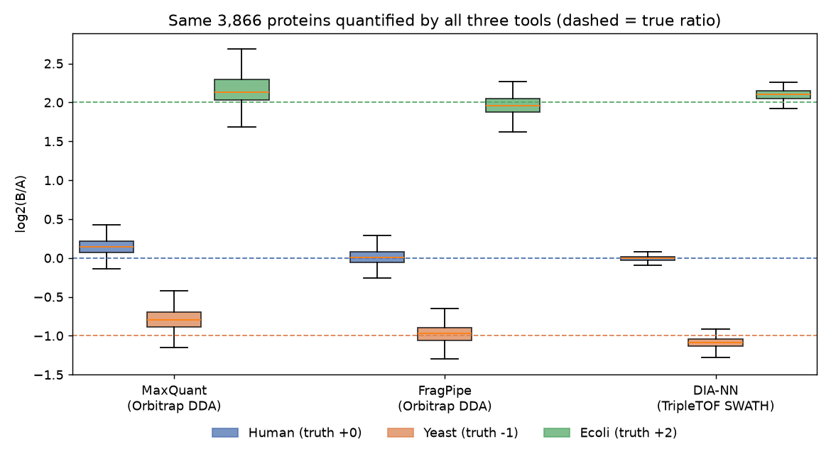Boxes show the middle 50% of proteins, whiskers the range without outliers; dashed lines are the true ratios.

Same 3,866 proteins	MaxQuant	FragPipe	DIA-NN
Human within ±0.5 (median)	98.9% (+0.14)	99.7% (+0.01)	100% (−0.01)
Yeast within ±0.5 (median)	92.4% (−0.80)	99.3% (−0.97)	99.4% (−1.09)
E. coli within ±0.5 (median)	80.9% (+2.13)	97.7% (+1.96)	97.7% (+2.10)
IQR human / yeast / E. coli	0.14 / 0.19 / 0.27	0.14 / 0.16 / 0.17	0.04 / 0.09 / 0.10

Three things stand out:

1. Precision. DIA-NN's ratios are much tighter. Its human IQR of 0.04 means the middle half of the unchanged proteins fell in a band 0.04 log2 units wide around zero.
2. Bias. MaxQuant compresses the yeast change (−0.80 instead of −1). DIA-NN slightly exaggerates both changes (−1.09, +2.10). FragPipe is closest on the medians. A small, consistent bias matters less than spread for finding changed proteins, but it matters if you report fold changes.
3. The extra proteins. The 1,760 proteins only DIA-NN quantified were less accurate: 94.3% of human, 87.1% of yeast and 67.4% of E. coli within ±0.5. That is the same pattern FragPipe showed: the proteins a tool adds at the edge of detection are its weakest.

Without match-between-runs

To see what MBR did, I re-summarised the first-pass results without --reanalyse by reusing the saved .quant files (--use-quant, 3 minutes):

DIA-NN	Human	Yeast	E. coli
MBR on	5,477 · 98.6%	2,374 · 95.1%	446 · 85.4%
MBR off	5,112 · 98.8%	1,923 · 96.2%	295 · 89.8%

MBR added 365 human, 451 yeast and 151 E. coli proteins at a small cost in accuracy, the same direction as in MaxQuant. Treat the MBR-off row as indicative: DIA-NN warns that reusing .quant files together with automatic mass-accuracy optimisation can give results that differ from a fresh run.

Traps I Hit

• The first-pass report has no protein quantities. In report-first-pass.parquet, PG.MaxLFQ is 0 for every row. If you want a no-MBR protein matrix from an MBR run, re-summarise with --use-quant as above, or run again without --reanalyse.
• "Use this mode for preliminary analyses only". With mass accuracy left on automatic, DIA-NN prints this. It optimised to 16 ppm (MS2) on the first run and recommended 13 ppm for MS1. For a final analysis, fix --mass-acc and --mass-acc-ms1 to values from a first run.
• Variable modifications switch on peptidoform scoring. Declaring Met oxidation prints a warning and enables it; add --no-peptidoforms if you do not want it.
• .wiff needs Windows. Calling the Windows diann.exe from WSL worked, with Windows paths for every file argument.

What This Does Not Show

• That DIA-NN beats MaxQuant or FragPipe as software. The DIA and DDA runs come from different instruments with different sensitivity and dynamic range. A fair software comparison needs DIA and DDA from the same instrument, or DDA software and DIA software on the same files where possible.
• Anything about other sample types. Three-species mixtures are clean and abundant. Low-input, plasma, PTM and single-cell work behave differently.
• Speed in general. Most of the 6 hours was reading SCIEX files twice.
• The best settings for each tool. I used common defaults. The DDA searches allowed two missed cleavages and N-terminal acetylation; the DIA-NN search did not.
• Statistical power. Three runs per condition. The scores describe accuracy of fold changes, not how many proteins a test would call significant; for that, see limma vs DEqMS at n = 3.

What I Would Take From It

• If you have a choice of acquisition, this dataset is a good argument for DIA: more proteins quantified, and fold changes about three times tighter on the proteins every workflow could measure.
• For any tool, the proteins only it quantifies are the ones to check before you trust them. Filtering on the number of valid values per condition helps; so does looking at how many precursors support each protein.
• Check bias as well as spread. A tool can be precise and still slightly over- or under-state fold changes.

Reproducing It

Commands, logs and the scoring scripts (score_diann.R, compare_three.R) are kept with the run, together with the per-run report.stats.tsv. The comparison uses the MaxQuant proteinGroups.txt and FragPipe combined_protein.tsv from the two earlier posts. Processing the DIA-NN output further in R is covered in After DIA-NN 2.x: report.parquet and pg_matrix, and the command-line basics in the DIA-NN tutorial.

References

• Van Puyvelde B. et al. (2022). A comprehensive LFQ benchmark dataset on modern day acquisition strategies in proteomics. Scientific Data 9:126. doi:10.1038/s41597-022-01216-6
• Demichev V. et al. (2020). DIA-NN: neural networks and interference correction enable deep proteome coverage in high throughput. Nature Methods 17:41–44. doi:10.1038/s41592-019-0638-x
• Cox J. et al. (2014). Accurate proteome-wide label-free quantification by delayed normalization and maximal peptide ratio extraction, termed MaxLFQ. Molecular & Cellular Proteomics 13:2513–2526. doi:10.1074/mcp.M113.031591