Correct Batch Effects, Then Test? With an Unbalanced Design, ComBat Turns a 5% False-Positive Target into 29%

Everything below comes from a simulation with a known answer and from a public Bioconductor data set with fake group labels. The script, its output and the figure are public, and CI re-runs the script and checks that it reproduces the published numbers exactly. No client data is used. (한국어판: 배치 보정하고 검정하면)

TL;DR

• A common workflow: correct batch effects with ComBat or removeBatchEffect, protecting the group variable, then run limma on the "clean" data.
• When groups are spread evenly over batches, this is close to fine: 5.5-6.3% of null genes reach p < 0.05 (target 5%).
• When groups are spread unevenly, it is not. With 11 of 12 samples of each group in one batch, 28-29% of null genes reach p < 0.05, and when 10% of genes really changed, 61-62% of the significant calls were false.
• Putting batch in the limma model (~ batch + group) stayed at 4.8-5.1% in every design. It loses power as the design gets more confounded, which is the honest price of the overlap.
• On a real data set (bladderbatch, 57 arrays in 5 batches) with fake labels, the corrected-then-tested route made 404-563 false discoveries per run at the strongest imbalance. Batch in the model made 0.4.

The workflow in question

Many pipelines look like this:

library(sva); library(limma)
clean <- ComBat(dat = expr, batch = batch, mod = model.matrix(~ group))   # protect group
fit   <- eBayes(lmFit(clean, model.matrix(~ group)))                     # then test group

or the same with removeBatchEffect(expr, batch = batch, design = model.matrix(~ group)). The corrected matrix looks clean on a PCA plot, so it feels safe to test it.

The problem was described by Nygaard, Rødland and Hovig (2016): when the correction "protects" the group effect, it uses the group labels to estimate the batch effect, and the test afterwards treats the corrected values as if they were measured that way. The uncertainty of the batch estimates, and the degrees of freedom they used, disappear from the test. limma's own help page says as much for removeBatchEffect:

"This function is intended for plotting and data exploration purposes. This function is not intended to be used to prepare data for linear modeling by 'lmFit'. For linear modeling, it is better to include the batch factors in the linear model..." (limma 3.58.1)

How much does it matter in practice? We measured it.

Setup

Five methods, each ending in limma lmFit + eBayes on the group coefficient, BH across genes:

Method	Before testing	Test model
ignore batch	nothing	~ group
batch in the model	nothing	~ batch + group
ComBat (group protected)	ComBat(mod = ~ group)	~ group
ComBat (batch only)	ComBat(mod = NULL)	~ group
removeBatchEffect (group protected)	removeBatchEffect(design = ~ group)	~ group

Simulation. 1,000 genes, two batches of 12 samples, 12 samples per group. Batch 1 holds k samples of group A and 12 - k of group B; batch 2 the reverse. So k = 6 is balanced (6:6) and k = 11 is nearly confounded (11:1). Every gene gets its own batch shift and batch scale. Two scenarios: no group effect at all (every call is false), and 10% of genes changed by ±1 log2. 40 repetitions per design.

Real data with a known null. The Bioconductor package bladderbatch: 57 bladder arrays in 5 batches (11/18/4/5/19), top 5,000 probes by mean. In each repetition we assign fake group labels at random within each batch, with a share p of group A in batches 1, 3 and 5 and 1 - p in batches 2 and 4. Given batch, the labels carry no biology, so every call is false. p = 0.5 is balanced; p = 0.9 is strongly unbalanced. 30 repetitions per p.

R 4.3.3, limma 3.58.1, sva 3.50.0.

Results

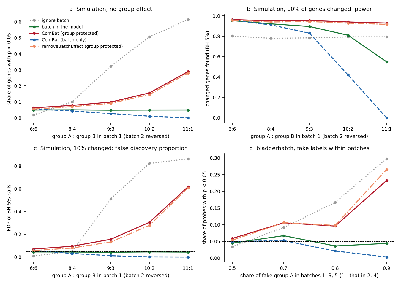Panels: a no group effect, share of p < 0.05 / b 10% of genes changed, power / c same, false discovery proportion / d bladderbatch with fake labels. The dashed line in a, c and d is the 0.05 target.

Simulation, no group effect: share of genes with p < 0.05 (should be 0.05)

Method	6:6	8:4	9:3	10:2	11:1
ignore batch	0.018	0.101	0.323	0.506	0.615
batch in the model	0.050	0.051	0.048	0.050	0.050
ComBat (group protected)	0.063	0.079	0.099	0.156	0.289
ComBat (batch only)	0.055	0.044	0.027	0.011	0.001
removeBatchEffect (group protected)	0.055	0.071	0.092	0.146	0.280

Simulation, 10% of genes changed: power and false discovery proportion at BH 5% (6:6 → 11:1)

Method	Power	FDP (target 0.05)
ignore batch	0.80 → 0.79	0.009 → 0.87
batch in the model	0.95 → 0.55	0.045 → 0.043
ComBat (group protected)	0.96 → 0.93	0.070 → 0.62
ComBat (batch only)	0.96 → 0	0.058 → 0
removeBatchEffect (group protected)	0.96 → 0.92	0.057 → 0.61

bladderbatch, fake labels: false BH discoveries per repetition (p = 0.5 → 0.9)

Method	False discoveries	Share of probes with p < 0.05
ignore batch	0 → 414	0.034 → 0.298
batch in the model	0.1 → 0.4	0.045 → 0.044
ComBat (group protected)	2.3 → 404	0.059 → 0.233
ComBat (batch only)	1.1 → 0	0.049 → 0.003
removeBatchEffect (group protected)	1.6 → 563	0.053 → 0.266

What the numbers say

1. Protected correction overstates confidence, and the worse the imbalance, the worse it gets. At 6:6 the inflation is small (5.5-6.3%). At 11:1 it is 28-29%, and most of the significant genes are false. The apparent power stays high (0.92-0.93) precisely because false calls are counted as finds.

2. Batch in the model is the method that keeps its promise. Its share of p < 0.05 stayed between 0.048 and 0.051 in every design, and its FDP between 0.042 and 0.045. Its power fell from 0.95 to 0.55 at 11:1. That drop is not a flaw: when almost all of group A sits in one batch, the data really contain less information to separate group from batch, and this is the only one of the five methods that admits it.

3. ComBat without the group (mod = NULL) fails the other way. It removes the batch difference, and with it the part of the group difference that overlaps with batch. It looks safe under the null and finds nothing at 11:1 (power 0).

4. In the simulation, ignoring batch is the worst of all with an unbalanced design, because the batch difference simply becomes a group difference (61% of null genes significant at 11:1).

5. Real data agree with the simulation. On bladderbatch with fake labels, both protected corrections made hundreds of false discoveries per run at p = 0.9. Batch in the model made fewer than one.

What to do instead

• For testing, put batch in the model. In limma: design <- model.matrix(~ batch + group), then lmFit, eBayes, and the group coefficient. In DESeq2 and edgeR the same idea is a design of ~ batch + group. This is what the limma help page above recommends.
• Use ComBat or removeBatchEffect for pictures, such as PCA plots and heatmaps, where nobody computes a p-value from the corrected values.
• Check your design before analysis. Tabulate group by batch. If the table is close to balanced, the methods behave similarly. If it is lopsided, expect batch-in-model to report fewer hits; that is the honest answer, not a weakness of the method.
• If group and batch are completely confounded (all of group A in batch 1), no method can separate them. The fix is in the experiment design, not the analysis.

From our own work

We asked the person who runs these analyses at sbmlab how this looks in practice (translated from Korean):

Samples that arrive in separate batches, experiments run on different days, and instrument time booked on different dates: it is hard to know how to analyse those together. I have used ComBat and several other R tools, RUV among them.

I do sometimes tell clients or collaborators "let's look at the design table first", but carefully. I did not run the experiment, so there is a limit to how much I can ask.

That last point is why the group-by-batch table is worth asking for early: it is a question about the data, not about how someone ran their lab. RUV-type methods, which estimate unwanted factors and add them to the model as covariates, are closer in spirit to "batch in the model"; we did not test them here.

Limits

• One simulation design (two batches, 12 samples each, per-gene batch shift and scale) and one real data set. Other designs, many small batches, or count data analysed directly with DESeq2 or edgeR may differ in size, though not in direction (Nygaard et al. report the same effect).
• 40 and 30 repetitions. The share of repetitions with any false BH call (in batch_study.out) has a 95% interval of about ±0.07-0.09, so single cells there are noisy; the trends over imbalance are clear.
• bladderbatch probes are correlated, so false discoveries per run are heavy-tailed. Read the trend over p, not single numbers. The correction methods dip between p = 0.7 and 0.8, and batch in the model reaches 0.067 at p = 0.7; we did not test why, and with 30 repetitions of correlated probes it is probably noise.

Reproduce it

Script, output, scores and figure: sbmlab-benchmarks/batch-correction-unbalanced. Rscript batch_study.R > batch_study.out takes a few minutes on R 4.3.3 with limma, sva and bladderbatch.

References

1. Nygaard V, Rødland EA, Hovig E. Methods that remove batch effects while retaining group differences may lead to exaggerated confidence in downstream analyses. Biostatistics 2016;17(1):29-39. doi:10.1093/biostatistics/kxv027
2. Johnson WE, Li C, Rabinovic A. Adjusting batch effects in microarray expression data using empirical Bayes methods. Biostatistics 2007;8(1):118-127. (ComBat)
3. Ritchie ME, et al. limma powers differential expression analyses for RNA-sequencing and microarray studies. Nucleic Acids Res 2015;43(7):e47.
4. Dyrskjøt L, et al. Gene expression in the urinary bladder: a common carcinoma in situ gene expression signature exists disregarding histopathological classification. Cancer Res 2004;64(11):4040-4048. (bladderbatch data)

Related

• Three samples per group: t-test vs limma
• Differential expression in proteomics: a complete R pipeline
• Missing values in proteomics: six imputation methods scored