STRING Confidence Score and Hub Proteins, Measured: What 0.4 vs 0.7 Changes and Whether Hubs Are Biology or Attention (STRING 12.5)

The STRING tutorial on this site shows how to get a network and an enrichment table out of STRING. The questions that come after it are harder: which confidence cut-off should I use, how far can I trust the "hub" proteins in the middle of the picture, and does a significant PPI enrichment p-value mean my list is biologically coherent?

I answered them with numbers rather than advice. Everything below uses STRING 12.5 (the current version, released September 2026) for Homo sapiens: the downloadable channel scores for the whole network, the STRING API for list-level tests, and a list of proteins actually detected by mass spectrometry.

Short answer

• The score is a calibrated probability, and it is reproducible. I recomputed every combined score from the seven channel scores with STRING's published formula, and all 5.4 million human pairs matched within rounding (±0.001).
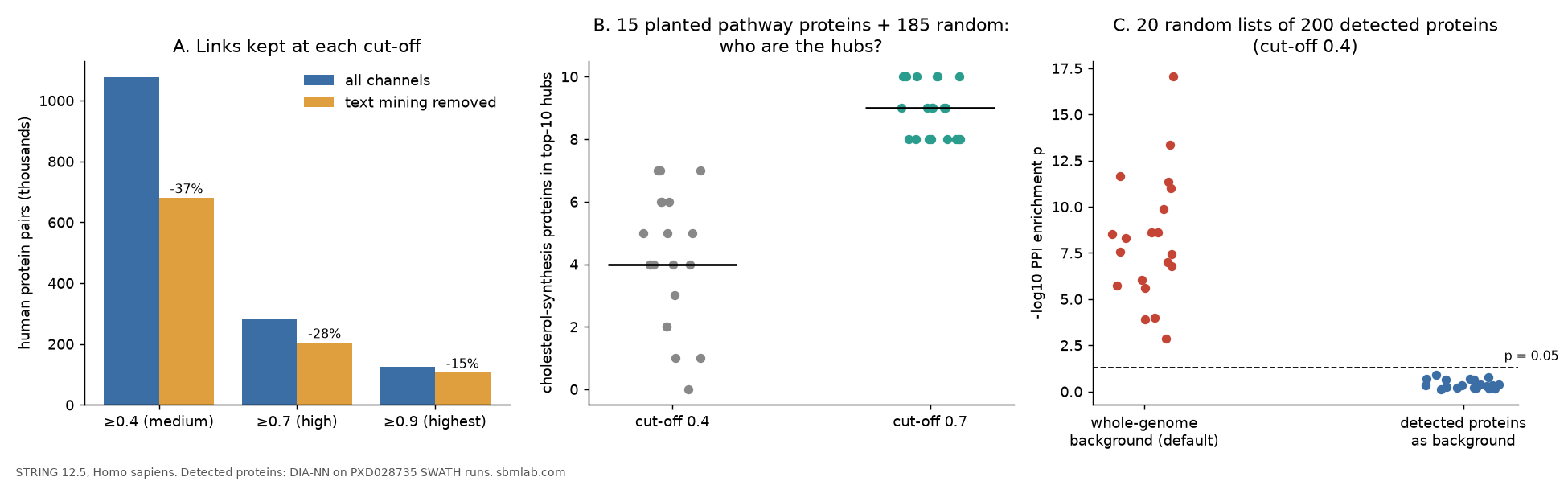
• At the default cut-off (0.4), 37% of human links depend on text mining. Remove the text-mining channel and they fall below 0.4. At 0.7 the figure is 28%, at 0.9 15%.
• At 0.4, the biggest hub in the human network is TRIM67, a protein with 17 PubMed records. 4,802 links, 97% of them carrying the same uniform experimental score of 0.457 and little else. Only 9 of them reach 0.7.
• Hubs are partly attention, but not only attention. Number of partners correlates with number of papers (Spearman 0.75 at 0.4). But among genes expressed in almost all cell lines, partner count separated core essential genes from the rest better than paper count did (AUC 0.83 vs 0.71), and it kept that power when papers were held constant.
• Random lists of detected proteins were "significantly connected" 20 times out of 20 with STRING's default whole-genome background, and 0 times out of 20 with the detected proteins as background. A real 15-protein pathway mixed into the lists stayed significant with either background.
• At 0.4 the hubs of a list were mostly well-studied bystanders; at 0.7 they were the real module. With 15 cholesterol-synthesis proteins planted among 185 random ones, they took a median of 4 of the top-10 hub positions at 0.4 and 9 of 10 at 0.7.

What the confidence score is

STRING's own papers define it precisely. The combined confidence score "correspond[s] to the estimated likelihood of a given association being true, given the underlying evidence", and it is calibrated against shared membership in KEGG pathway maps (Szklarczyk et al. 2023). The 2025 paper repeats that the scores "describe the estimated likelihood of a postulated association being correct" (Szklarczyk et al. 2025).

Two consequences follow. A score of 0.7 is not "70% binding strength"; it is how confident STRING is that the two proteins are functionally associated, which includes being in the same pathway without ever touching. And STRING's help pages name the cut-offs: low 0.15, medium 0.4 (the web default), high 0.7, highest 0.9. On how to choose, the FAQ is honest: "You have to choose some arbitrary number based on the number of interactions you need for you [sic] analysis."

Reproducing the score

Each pair has seven channel scores: neighborhood, fusion, co-occurrence, co-expression, experiments, databases and text mining. STRING removes a prior (p = 0.041) from each, combines them as independent evidence, and adds the prior back once (STRING FAQ; von Mering et al. 2005):

import numpy as np, pandas as pd

PRIOR = 0.041
CH = ["neighborhood", "fusion", "cooccurence", "coexpression",
      "experimental", "database", "textmining"]

def combine(df, chans):
    one_minus = np.ones(len(df))
    for c in chans:
        s = df[c].to_numpy() / 1000.0
        s = np.where(s < PRIOR, PRIOR, s)
        one_minus *= 1.0 - (s - PRIOR) / (1 - PRIOR)
    return np.floor(((1.0 - one_minus) * (1 - PRIOR) + PRIOR) * 1000).astype(int)

L = pd.read_csv("9606.protein.links.detailed.v12.5.txt.gz", sep=" ")
L = L[L.protein1 < L.protein2]                      # each pair is listed twice
L["recomputed"] = combine(L, CH)
L["no_textmining"] = combine(L, [c for c in CH if c != "textmining"])
print((L.recomputed - L.combined_score).abs().max())  # 1

On the 5,413,027 human pairs in the file, 86.4% matched exactly and 100% matched within 1 (on the 0–1000 scale). The detailed file's channel scores already merge direct and transferred (orthology) evidence, which is why a small share differs by the rounding step. So the same function with the text-mining channel left out gives a formula-level "without text mining" score. It is a counterfactual, not a clean separation: curated databases and experiment records are themselves partly built from the literature.

How much of the network is text mining?

Cut-off	Human pairs	Without text mining	Lost	Text mining is the only channel
≥ 0.4 (medium)	1,076,224	680,472	37%	8.8%
≥ 0.7 (high)	282,864	204,623	28%	3.2%
≥ 0.9 (highest)	125,344	106,437	15%	0.5%

Two different numbers matter here. Only 8.8% of 0.4-level links have text mining as their only evidence, but 37% need it to reach 0.4. The other 28% have some co-expression, experimental or other support that is too weak on its own and that text mining tops up. Text mining counts co-mentions of protein names in the literature (Szklarczyk et al. 2025), so it carries whatever the literature pays attention to. Higher cut-offs lean more on curated databases and experiments: the share of links with experimental or database evidence rises from 69.5% at 0.4 to 96.0% at 0.9.

The hub made of one kind of evidence

Sorting proteins by number of partners at 0.4 gives this top three:

Protein	Partners at ≥ 0.4	Partners at ≥ 0.7	Links whose experimental score is exactly 0.457	PubMed records
TRIM67	4,802	9	97.2%	17
ZRANB1	4,071	160	93.5%	53
PLEKHA4	2,945	7	85.6%	20
TP53 (for comparison)	2,396	872	9.3%	20,405

Thousands of links with the same experimental score, almost no other evidence, and nearly all gone at 0.7: that is what high-throughput interaction data look like after scoring. The value itself does not identify a source. Across the human network, 120,470 pairs have an experimental score of exactly 0.457, spread over 13,770 proteins; 264 proteins have at least 100 such links and 49 have at least 500 (after TRIM67, ZRANB1, VIRMA and PLEKHA4 come UBE2H, CDC123, KIF14, TIPARP and HNRNPL). I did not trace which datasets lie behind them, so I won't name any. Overall, 72,871 links at ≥ 0.4 (6.8%) rest on the experimental channel alone, and 32,091 of those have exactly 0.457.

The practical point is that at 0.4 one kind of uniformly scored high-throughput evidence can make an obscure protein the most connected node in your picture. At 0.7 most top hubs become what you would expect: TP53, histone H4, the ubiquitin precursors RPS27A, UBA52 and UBC, MAPT, β-actin. Not all of them, though: ANLN is seventh at 0.7 with 571 partners and 171 PubMed records, and has 1,052 links at exactly 0.457. A higher cut-off reduces this effect; it does not remove it.

Are hubs essential, or just well studied?

The idea that highly connected proteins are more often essential goes back to Jeong et al. (2001) in yeast, and He and Zhang (2006) argued it arises because hubs take part in more essential protein–protein interactions. The worry is that interaction databases mirror research attention: Haynes et al. (2018) showed that gene annotation is concentrated on genes that were already well studied, and Gillis and Pavlidis (2011) showed that multifunctionality, which is encoded in how connected a gene is, can by itself drive much of the apparent performance of network-based function prediction.

I tested both at once. For each protein I counted its partners in STRING and its PubMed records in NCBI's gene2pubmed, and labelled genes with the Hart et al. (2017) core-essential list (CEGv2) from CRISPR screens.

Partners and papers go together. The Spearman correlation between number of partners and number of PubMed records was 0.75 at 0.4, 0.69 at 0.7, and 0.60 at 0.7 with text mining removed. The 100 biggest hubs at 0.4 had a median of 762 PubMed records, against 54 for all proteins.

But essential genes are hubs beyond what papers explain. The obvious comparison, Hart's essential genes against the non-essential reference list NEGv1 (Hart et al. 2014), gives an AUC of 0.94 for partner count. That number is inflated: the non-essential reference genes were chosen as genes not expressed in cell lines, so they have little co-expression or interaction data to begin with. A fairer comparison keeps only genes that the Human Protein Atlas detects (nTPM ≥ 1) in at least 90% of its cell lines (9,087 genes, 8,917 of which mapped to STRING and NCBI), and compares the 665 core-essential genes among them with the 8,252 others:

Predicting core-essential genes among broadly expressed genes	AUC
PubMed records	0.71
Partners at ≥ 0.4	0.81
Partners at ≥ 0.7	0.83
Partners at ≥ 0.7, text mining removed	0.82

In a logistic model with both log partner count and log paper count, partners kept a large coefficient (1.68 per standard deviation at 0.7), while papers became slightly negative (−0.15; 0.01 with text mining removed). Within thirds of the publication distribution, partner count at 0.7 still separated essential from other genes with an AUC of 0.77 to 0.80, while paper count within the same thirds managed only 0.54 to 0.65.

A network biologist will ask about expression: essential genes are highly expressed, and abundant proteins collect pull-down partners. Mean expression across the HPA cell lines did predict essentiality (AUC 0.73), but within each fifth of the expression distribution partner count still gave AUCs of 0.77 to 0.79, and adding log expression to the model kept the partner coefficient at 1.50. The "others" include essential genes that are not on Hart's core list, so these numbers are conservative.

So hubs are not just famous proteins. They are a mixture: real biological centrality, plus a layer of attention that grows at low cut-offs and with text mining.

What happens when you paste your own list

The network-wide numbers matter because of what STRING does with a list. I took the 5,560 human proteins in DIA-NN's protein-group matrix (pg_matrix, 1% protein-group FDR) from a public benchmark (Van Puyvelde et al. 2022, the SWATH runs used in the DIA-NN benchmark) and sent lists of 200 to the STRING API's ppi_enrichment endpoint.

Random lists of detected proteins. Twenty random draws of 200 proteins, no biology behind them:

	p < 0.05 (out of 20)	Median p	Observed / expected links
Cut-off 0.4, whole-genome background (default)	20	1.7 × 10⁻⁸	1.29
Cut-off 0.7, whole-genome background	17	9.2 × 10⁻⁴	1.29
Cut-off 0.4, detected proteins as background	0	0.47	1.00
Cut-off 0.7, detected proteins as background	0	0.49	1.00

Proteins that a mass spectrometer detects are broadly expressed and well studied: 92% of this detected set is expressed in at least 90% of HPA cell lines (45% of all STRING proteins), and its median is 113 PubMed records (54 for all proteins). So any set of them has about 30% more links than a random set of genome proteins. STRING's Getting started page does warn that "enrichment is to be expected" in some cases and that the numbers "have to be interpreted with some caution"; the measured version of that warning is 20 out of 20. It is the network counterpart of the background trap in STRING's GO enrichment.

A real pathway hidden in the noise. Twenty lists of 15 of the 17 detected cholesterol-biosynthesis proteins (Reactome R-HSA-191273), drawn at random, plus 185 random detected proteins. A curated metabolic pathway is a favourable case for STRING, since such pathways are part of how its scores are calibrated:

	p < 0.05 (out of 20)	Median observed / expected
Cut-off 0.4, whole-genome background	20	1.59
Cut-off 0.4, detected background	20	1.26
Cut-off 0.7, detected background	20	1.59

The right background did not cost the real signal anything.

Who are the hubs of that list? Counting partners inside each 200-protein list, the 15 planted proteins took a median of 4 of the top-10 positions at 0.4 (range 0 to 7) and 9 of 10 at 0.7 (range 8 to 10). In the first list, the top three at 0.4 were BRD4, TRIM28 and YBX1, each with 777 to 1,816 PubMed records; at 0.7 BRD4 stayed first, followed by nine cholesterol-synthesis enzymes. In the random lists, the three biggest in-list hubs had a median of 340 PubMed records.

To pass the background through the API:

import json, urllib.parse, urllib.request

def ppi_enrichment(ids, background, score=400):
    data = {"identifiers": "%0d".join(ids), "species": 9606, "required_score": score,
            "background_string_identifiers": "%0d".join(background),
            "caller_identity": "your_lab"}
    req = urllib.request.Request("https://version-12-5.string-db.org/api/json/ppi_enrichment",
                                 data=urllib.parse.urlencode(data).encode())
    with urllib.request.urlopen(req, timeout=120) as r:
        return json.load(r)[0]   # number_of_edges, expected_number_of_edges, p_value

In R, STRINGdb$set_background() does the same for the package's enrichment functions.

What I would do with this

• Use 0.7 for hub-centric conclusions. At 0.4 one kind of uniformly scored high-throughput evidence or a pile of co-mentions can create a top hub. If you show a 0.4 network, say so and check the top hubs at 0.7.
• Look at the evidence channels of the hubs you plan to write about. Click the edge in STRING or read the channel columns from the download. A hub supported by one experimental score is a lead, not a result.
• Always pass your detected proteins as the background for PPI enrichment, as for GO enrichment. With the whole genome as background, "significantly connected" is the expected result for a typical proteomics list.
• Treat "my list is significantly connected" as weak evidence. Our random lists were 29% over expectation with the default settings. A real 15-protein module pushed that to 59%.
• Turning text mining off is a sensitivity check, not a fix. It removed 37% of links at 0.4, yet the correlation between partners and papers only fell from 0.75 to 0.65 (0.60 at 0.7). Attention reaches the network through the other channels too.

Limitations

• Human only, STRING 12.5 only. Other organisms have very different channel mixes; text mining changes between versions (Szklarczyk et al. 2023 reports a twofold increase in text-mined physical pairs, across all organisms, from 11.5 to 12.0).
• Essentiality is a proxy for "biologically central". Hart's core-essential genes are mostly housekeeping machinery (ribosome, proteasome, spliceosome), which is densely connected and densely studied at the same time. "Broadly expressed" was defined by one threshold on Human Protein Atlas cell-line RNA (1,206 cell lines; the file inside the download is dated May 2023).
• PubMed records are a proxy for attention. gene2pubmed links papers to genes with varying depth; it is not a count of papers about each gene.
• One detected proteome. The random lists came from one SWATH experiment on one cell-line mixture. Other tissues detect different proteins, but the reason detected sets are over-connected (abundance and attention) is general.
• Gene symbols, not identifiers, were used to join STRING to NCBI and to the detected list; 19,315 of 19,699 STRING proteins mapped to an NCBI gene.

Code and outputs: the scripts (network recomputation, hubs and essentiality, API lists, figure) and their JSON outputs are in sbmlab-benchmarks/string-hubs. The STRING, NCBI and HPA files are public downloads and are not copied there.

Related

• STRING Database Tutorial (v12): getting networks and enrichment out of STRING in R and on the web
• STRING enrichment and the background trap: the same problem for GO and KEGG terms
• PPI network hub analysis: centrality measures and how they are computed

References

• Szklarczyk D. et al. (2025). The STRING database in 2025: protein networks with directionality of regulation. Nucleic Acids Research 53:D730–D737. doi:10.1093/nar/gkae1113
• Szklarczyk D. et al. (2023). The STRING database in 2023: protein–protein association networks and functional enrichment analyses for any sequenced genome of interest. Nucleic Acids Research 51:D638–D646. doi:10.1093/nar/gkac1000
• von Mering C. et al. (2005). STRING: known and predicted protein–protein associations, integrated and transferred across organisms. Nucleic Acids Research 33:D433–D437. doi:10.1093/nar/gki005
• Jeong H., Mason S.P., Barabási A.-L., Oltvai Z.N. (2001). Lethality and centrality in protein networks. Nature 411:41–42. doi:10.1038/35075138
• He X., Zhang J. (2006). Why do hubs tend to be essential in protein networks? PLoS Genetics 2:e88. doi:10.1371/journal.pgen.0020088
• Haynes W.A., Tomczak A., Khatri P. (2018). Gene annotation bias impedes biomedical research. Scientific Reports 8:1362. doi:10.1038/s41598-018-19333-x
• Gillis J., Pavlidis P. (2011). The impact of multifunctional genes on "guilt by association" analysis. PLoS ONE 6:e17258. doi:10.1371/journal.pone.0017258
• Hart T. et al. (2014). Measuring error rates in genomic perturbation screens: gold standards for human functional genomics. Molecular Systems Biology 10:733. doi:10.15252/msb.20145216
• Hart T. et al. (2017). Evaluation and design of genome-wide CRISPR/SpCas9 knockout screens. G3 7:2719–2727. doi:10.1534/g3.117.041277
• Van Puyvelde B. et al. (2022). A comprehensive LFQ benchmark dataset on modern day acquisition strategies in proteomics. Scientific Data 9:126. doi:10.1038/s41597-022-01216-6
• STRING help pages (FAQ, Getting started, API), accessed 19 October 2026. string-db.org/help
• Human Protein Atlas, cell line RNA expression (rna_celline.tsv, downloaded 19 October 2026; data file dated 24 May 2023, 1,206 cell lines). proteinatlas.org
• NCBI Gene: gene2pubmed and Homo_sapiens.gene_info, downloaded 19 October 2026. ftp.ncbi.nlm.nih.gov/gene/DATA