Does WGCNA Really Work? Running It End to End on Public Proteomics Data

WGCNA (weighted gene co-expression network analysis) is one of the most widely used methods in omics papers. The typical flow is: find modules → pick the module linked to a trait → present its hub genes as key targets. We ran that flow end to end on public data. Along the way we changed the intermediate settings, cut the sample size, re-checked the modules in another cohort, and compared them with random protein sets. Our conclusion: WGCNA is good at finding groups of molecules that move together. It is weaker than expected at finding the genes that explain a trait. Everything below uses public data (CPTAC renal cancer · TJ-RCC) and published literature only. No client data is used. (한국어판: WGCNA는 정말 효과가 있을까)

---

Students who hang out together

Suppose you record who walks around with whom at a school and split the students into "groups." Groups will certainly appear. But did they form because the students are friends?

• They may live in the same neighbourhood and take the same bus,
• they may belong to the same club,
• or they may genuinely get along.

And if you find "the group with good grades," there is no guarantee that its most popular member is the one raising the grades.

WGCNA modules and hubs are the same. Modules always appear. The questions are what made them, and whether their link to a trait is better than any random group.

---

What we did

Item	Details
Discovery cohort	CPTAC clear-cell renal carcinoma, 110 tumours, proteome · histologic grade G1 7 · G2 51 · G3 41 · G4 11
Replication cohort	TJ-RCC, 100 tumours, proteome (different country, instrument and processing)
Proteins	Shared by both cohorts with ≤10% missing (exact zeros in TJ-RCC treated as missing); top 3,000 by variance in the discovery cohort
Baseline settings	Module-cutting values from the WGCNA tutorial (minModuleSize 30 · deepSplit 2 · mergeCutHeight 0.25), with a signed network and power 10 (the first power reaching scale-free fit R² 0.80). The tutorial itself uses an unsigned network at power 6.
Experiments	① change one setting at a time ② subsample ③ re-check in another cohort and another molecular layer ④ compare with size-matched random sets ⑤ identify modules with cell-type markers ⑥ compare prediction performance

We used tumours only, for a reason. Mixing tumour and normal tissue pulls the modules toward "tumour vs normal." Running the same pipeline on the replication cohort with its normals included (TJ-RCC, 100 tumours + 50 normals) gave two largest modules correlated with tumour status at r −0.82 and 0.74. Already 47.5% and 27.5% of their proteins were differentially expressed. When the design has a large group difference, WGCNA mostly repeats the differential analysis.

---

1. The good news — modules are real "groups"

• All 15 modules were enriched for GO biological processes. Only 5% of 200 random protein sets of the same sizes were.
• Groups that are "made together and work together" separated cleanly: mitochondrial respiration, ribosomes, RNA splicing, complement and extracellular matrix.
• In a cohort measured in another country on another instrument, 12 of 15 modules were preserved above size-matched random modules.

So as a tool for showing the structure of a dataset, WGCNA does its job.

---

2. Intermediate settings — where results diverge

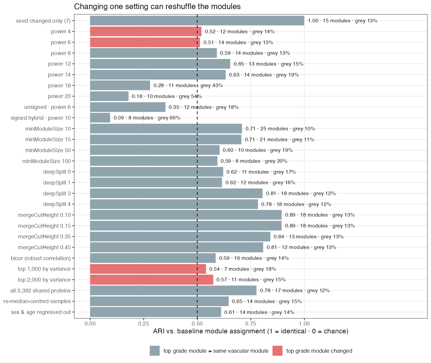
Each bar shows agreement with the baseline run: were the same proteins put in the same module (ARI, 1 = identical · 0 = chance)? Red bars mark runs where "the module most associated with grade" became a different module. In those runs, the conclusion sentence of a paper would change.

• Soft power. On the same curve (the tutorial's candidate powers, 1–10 then even numbers to 20), a scale-free fit cut-off of R² 0.80 gives power 10, 0.85 gives 18 and 0.90 gives 20. The package's automatic estimate is 18. (Scanning every integer power instead gives 17 and 19.) At power 18 the mean connectivity drops to about 2, and 43% of proteins fall into no module at all. Going the other way, at power 4 or 6 "the module most associated with grade" itself became a different module.
• Network type. An unsigned network (at its customary power 6) drops agreement to 0.35, and signed hybrid (at power 10) to 0.09. It is effectively a different analysis.
• Input set. With only the top 1,000 proteins by variance, the "grade module" becomes an immune module. With the top 2,000, it becomes an ER/Golgi module.
• How finely modules are cut (minModuleSize · deepSplit · mergeCutHeight) mattered less. The number of modules changed, but the large groups stayed.

The rationale for choosing power by scale-free fit is weak in itself. A survey of 928 real networks found the strongest level of evidence for scale-free structure in only 4% [1]. In a test of how well RNA-seq co-expression networks predict gene function (GO), soft thresholding lowered performance relative to plain correlation [2]:

"Also, the WGCNA soft thresholding acts in a similar fashion, lowering performance (average AUROC = 0.55)."

In short, the input set, the power and the network type change the result. Report their values with the reason for each choice, and show that the conclusion holds under two or three alternatives.

---

3. Sample size — how many is enough?

We drew n samples out of 110, 20 times each.

Samples	Agreement with full result (ARI)	Strongest correlation with grade	"Grade module found" rate (p < 0.05)
15	0.19	0.66	75%
20	0.24	0.59	95%
30	0.29	0.57	90%
60	0.43	0.47	100%
80	0.48	0.49	100%

(Strongest correlation with all 110 samples = 0.46)

With 15 samples the module assignment is essentially a different result. Yet the correlation is inflated from 0.46 to 0.66, and three runs out of four would still report "a module linked to grade." This is the winner's curse of picking "the strongest" in a small sample. The package authors also advise against fewer than 15 samples and recommend at least 20 if at all possible [3].

---

4. Trait-linked modules — compared with random sets

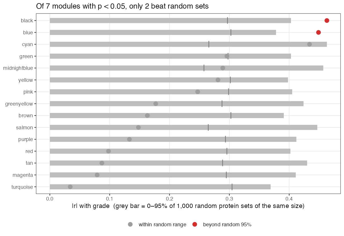
The textbook approach correlates each module eigengene with grade and takes the p-value. By that test, 7 modules were significantly associated with grade.

But draw random protein sets of the same size 1,000 times and do the same calculation, and they also reach |r| ≈ 0.30 with grade. Grade is one of the major axes of the data, so averaging almost any proteins partly captures that axis.

Only 2 modules exceeded this random benchmark. The grey bars show the 95% range of the random sets.

A module–trait p-value only tests "the correlation is not zero." It does not test "better than any random set."

---

5. What the top module really is — vascular content

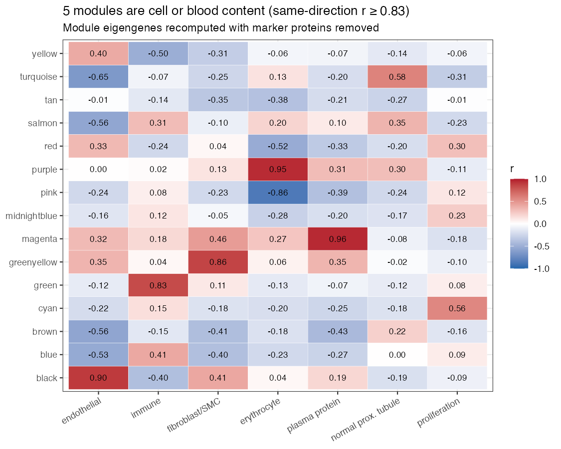
The hubs of the module most associated with grade (r −0.46) were RASIP1, CDH13, PLVAP and similar proteins. We built an endothelial score from standard endothelial markers chosen without looking at the modules (PECAM1, VWF, CDH5, ENG, EMCN, ESAM). The module correlated with it at r 0.90. Four of these markers are also members of the module; removing them from the module and recomputing gave the same result. Adjusting for that score shrank the grade correlation from −0.46 to −0.21 (still p ≈ 0.03, so shrunk rather than gone).

So "higher grade, lower module" is true. But it reflects the proportion of blood vessels in the tissue more than a regulatory change inside tumour cells.

This is not unique to this dataset. Five of 15 modules were cell or blood content: immune, vascular, stromal, erythrocyte and plasma. A study of brain and blood transcriptomes (RNA) concluded [4]:

"Our conclusion is that the dominant coexpression signal in brain, blood, and, likely, other complex tissues can be attributed to cellular compositional effects, rather than intra-cell-type regulatory relationships."

Proteomics adds one more trap. The plasma-protein and erythrocyte modules did not reappear in RNA from the same patients. These are proteins that came in with the blood, not proteins the tissue made. Interpreting them as "regulatory programmes" is wrong.

---

6. The module preservation score trap

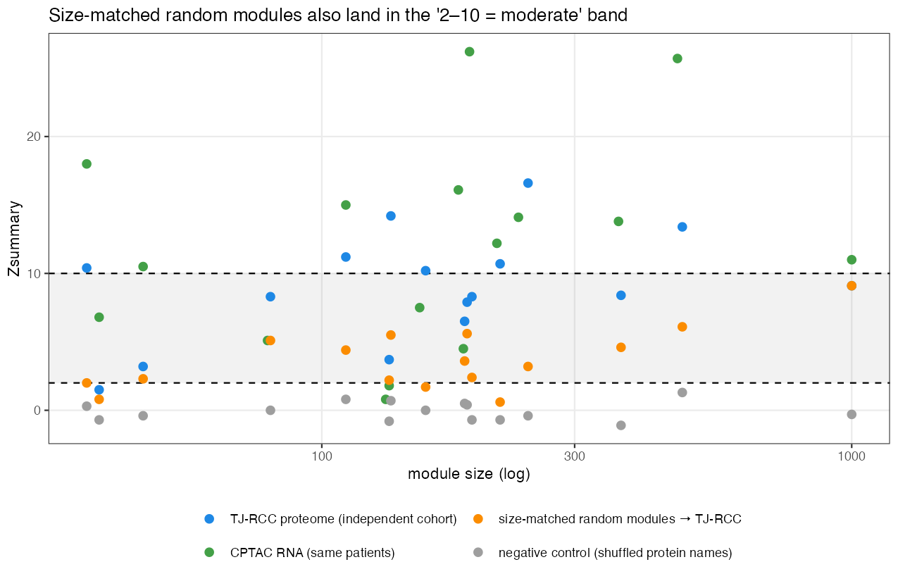
Zsummary, the standard index for whether a module exists in other data, comes with widely used thresholds [5]:

"…if [Zsummary > 10] there is strong evidence that the module is preserved; if [2 < Zsummary < 10] there is weak to moderate evidence of preservation; if [Zsummary < 2], there is no evidence that the module preserved."

We then built random modules of the same sizes by shuffling the module labels across proteins. 12 of 15 scored Z ≥ 2 (maximum 6.1). A random 1,000-protein set scored 9.1. A negative control with shuffled protein names scored −1.1 to 1.3, so the tool itself works correctly.

The same paper notes that Z grows with module size [5]. Random sets also fall into the "2–10 = moderate" band. Always show size-matched random modules alongside the real ones.

---

7. Hub genes and prediction

Hubs are stable, but stable does not mean important. With 30 samples, 6 of the top-10 hubs reappeared. For comparison, only 1 of the 10 proteins most correlated with grade reappeared. A hub is "the protein moving most like the module average," so it averages away noise. But the hubs of the vascular module above were simply vascular markers.

Two of the WGCNA authors wrote [6]:

"While there is an ongoing debate in the literature regarding the importance of hub genes, it is fair to say hubs are often not important."

In the very next sentence they argue for focusing on hubs within modules rather than hubs of the whole network, which is the kind of hub used here.

"…while network methods may be preferable when learning about biology, standard marginal meta-analysis methods may be better suited for selecting candidate biomarkers."

Modules did not predict better either. We compared cross-validated AUC for predicting high grade (G3–4):

Predictor	AUC
Score from the top 50 grade-correlated proteins	0.73
15 principal components	0.72
15 module eigengenes	0.70

Modules are "easier-to-read principal components," not "stronger" ones. A benchmark of 42 methods also found that decomposition methods (ICA variants) recovered known regulatory modules best [7]. To be fair, the same benchmark ranked WGCNA among the best of the clustering methods.

---

8. What we do

• Below 20 samples we do not recommend WGCNA. Between 20 and 30 we use it to explore structure only, and we draw module–trait conclusions from 30 samples upward.
• Designs with large group differences (tumour/normal and similar) are analysed within groups.
• We report the power, network type and input set with their reasons, and we re-run with two or three alternatives to show whether the conclusion holds.
• Every module gets GO results plus its correlation with cell and blood markers. Plasma and erythrocyte modules are flagged separately.
• Module–trait associations come with a comparison against size-matched random sets. Preservation scores come with size-matched random modules.
• Hubs are delivered as candidates only.

---

Closing

WGCNA is a good map of the groups that exist in your data. It shows large axes such as cell composition, blood carry-over and batch at a glance, and it reduces thousands of variables to a few dozen scores.

But a line on a map is not yet a road. If a module is linked to a trait, ask first: is it better than any random set? Then ask: is it just cell composition? Only after both questions does a hub become a "candidate to validate" — not a "key gene."

Reproduce it

wgcna-cptac-ccrcc downloads the public inputs (about 48 MB) and re-runs the main numbers in about 4.5 minutes: the module count, the 7 vs 2 grade-linked modules, the vascular module and its adjustment, and the three AUCs. It was written separately from the original analysis, from the settings stated above only, and the numbers came back to the second decimal (R 4.3.3, WGCNA 1.74). It also shows that the count of 7 depends on preprocessing: keeping TJ-RCC zeros as values gives 3, a CPTAC-only filter gives 2. The vascular module stays the strongest, and only 2–3 modules beat random sets, in every variant. GO enrichment, preservation scores, the subsampling table and the per-setting bars were not re-run.

---

References

1. Broido AD, Clauset A. Scale-free networks are rare. Nature Communications 2019;10:1017. doi:10.1038/s41467-019-08746-5
2. Ballouz S, Verleyen W, Gillis J. Guidance for RNA-seq co-expression network construction and analysis: safety in numbers. Bioinformatics 2015;31(13):2123–2130. doi:10.1093/bioinformatics/btv118
3. Langfelder P, Horvath S. WGCNA package: Frequently Asked Questions. (web document, updated Dec 2017) https://horvath.genetics.ucla.edu/html/CoexpressionNetwork/Rpackages/WGCNA/faq.html (archived copy; the live site currently shows a certificate warning)
4. Farahbod M, Pavlidis P. Untangling the effects of cellular composition on coexpression analysis. Genome Research 2020;30(6):849–859. doi:10.1101/gr.256735.119
5. Langfelder P, Luo R, Oldham MC, Horvath S. Is my network module preserved and reproducible? PLoS Computational Biology 2011;7(1):e1001057. doi:10.1371/journal.pcbi.1001057
6. Langfelder P, Mischel PS, Horvath S. When is hub gene selection better than standard meta-analysis? PLoS ONE 2013;8(4):e61505. doi:10.1371/journal.pone.0061505
7. Saelens W, Cannoodt R, Saeys Y. A comprehensive evaluation of module detection methods for gene expression data. Nature Communications 2018;9:1090. doi:10.1038/s41467-018-03424-4

All quoted sentences were checked against the original papers or documents (the quote from [4] is from its abstract). Data: CPTAC clear-cell renal carcinoma proteome (Clark DJ et al. Cell 2019;179(4):964–983.e31, doi:10.1016/j.cell.2019.10.007; LinkedOmics processed matrices) and TJ-RCC (Hu J et al. Nature Genetics 2024;56(3):442–457, doi:10.1038/s41588-024-01662-5; Zenodo 8063124, CC-BY-4.0). Tool: R WGCNA 1.73. We focused on a single trait (histologic grade). Each cell-type score is the mean of 4–7 markers. The same numbers should not be assumed for other tissues, metabolomics data or other traits.