Zero Proteins Passed FDR: How to Read and Report a Null Result (DIA-NN Reanalysis, 70 Placentas)

Read this first. This post is about my downstream workflow: what I did after DIA-NN when the statistics came back empty. I use a public dataset as the worked example, and the group labels are just labels here. It is not a study of depression or antidepressants, the biological and clinical questions are outside its scope, and it makes no comparison with the published study the data come from. Nothing here says whether any medication is safe or unsafe in pregnancy; decisions about medication belong with a doctor.

When the Statistics Come Back Empty

In the previous post I ran DIA-NN 2.3.2 on 210 public SWATH runs (PRIDE PXD071192) and cleaned the protein matrix down to something analysable. The next step was the one everyone runs for: differential expression.

The answer, in all three comparisons: zero proteins pass a 5% false discovery rate. The closest one sits at FDR 0.39.

Most tutorials stop before this happens to you, so there is not much written about what to do next. The temptation is to loosen something until a list appears. This post is the other option: read the null properly, say what it does and does not rule out, and report it so a reader can use it.

What Was Run

• Matrix: protein groups at 1% global protein-group FDR from report.parquet, contaminants removed — 1,720 groups (how and why: previous post)
• Replicates: the three injections of each placenta averaged on the log2 scale → 70 biological samples
• Filter: a protein is tested in a comparison only if quantified in at least 60% of the samples in both groups
• No imputation
• Test: limma, eBayes(trend = TRUE, robust = TRUE), Benjamini–Hochberg FDR

Comparison	n (placentas)	Proteins tested	Pass FDR 5%	Lowest FDR
Depression without SRI vs control	34 vs 18	1,603	0	0.39
Depression with SRI vs without	18 vs 34	1,604	0	0.99
Depression with SRI vs control	18 vs 18	1,617	0	0.76

Adding infant sex, gestational age and maternal age as covariates did not change the count: still 0 in every comparison. The unfiltered matrix as DIA-NN wrote it gave the same: 0 passing, lowest FDR 0.405. I reran every number above independently from the same files before writing them down.

Step 1: Look at the p-value Histogram Before Anything Else

The FDR count tells you how many proteins crossed a line. The p-value histogram tells you why. Plot the raw p-values in 20 bins and compare each bar to what you would expect if no protein differed at all — a flat line at (proteins tested ÷ 20).

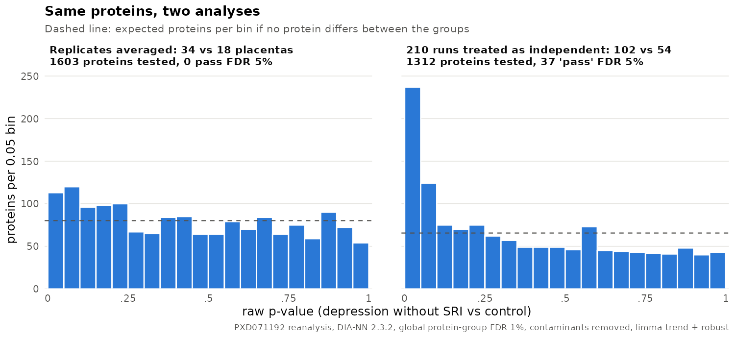
The left panel at the top of this post is the correct analysis. What it shows:

• Mostly flat. If the groups differed broadly, the left-most bars would tower over the rest. They don't.
• A small excess near zero. 113 proteins have a raw p below 0.05, where chance alone predicts about 80. limma::propTrueNull() puts the share of truly unchanged proteins at about 0.91.
• Nothing tall enough to survive correction. A modest bulge spread over many proteins is exactly the pattern FDR cannot turn into individual hits.

So the honest reading for this comparison is not "nothing is there". It is "if something differs, it is small and spread out — no single protein stands out from the noise."

The other two comparisons are flatter still. For SRI vs no SRI there are 56 proteins below 0.05 against roughly 80 expected — fewer than chance — and the estimated null share is 1.0.

Adjusting for the three covariates shrinks the excess in the first comparison from 113 to 88. Some of the bulge was tracking things other than the group label.

The right panel: how to get 37 "hits" from the same data

Now treat the 210 injections as 210 independent samples (102 vs 54), which is the most common mistake with technical replicates. Same proteins, same test:

	Replicates averaged (correct)	210 runs as independent
Raw p below 0.05	113 (≈80 expected)	237 (≈66 expected)
Pass FDR 5%	0	37
Lowest FDR	0.39	0.004

Nothing about the biology changed. The three injections of one placenta agree with each other much more than two placentas do, and counting them separately tells the model it has three times the evidence it really has. The spike in the right panel is that error made visible — and if you ever see a histogram like that from a design with replicates, check how the replicates were handled before you believe it. The fixes are in the previous post.

Step 2: Don't Go Looking for a List

Every way of producing a list from this result is a way of forgetting the FDR:

• Raw p below 0.1. In the first comparison that is 233 proteins. Chance alone predicts about 160. Most of the list is noise, and you cannot tell which part isn't.
• Ranking the "top 20" and naming them. The top of a null list is still a null list. Once a table of gene names appears in a report, someone will quote it as a finding.
• Enrichment on the raw-p list. GO or KEGG analysis on a list that is mostly noise returns terms that are mostly noise, with very convincing names. If a pipeline needs a demonstration figure, every panel needs an "exploratory, not significant" label on it.
• Switching test or normalisation until something passes. Each switch is another look at the same data.

An exploratory list is legitimate only if it is labelled as one, ranked by something honest, and kept away from the results section.

Step 3: Say What the Data Rule Out

"No significant difference" is a weak sentence. A null result becomes useful when you state how large an effect the data are incompatible with. The tool for that is the 95% confidence interval of each log2 fold change, which limma gives you directly:

tt <- topTable(fit, coef = 2, number = Inf, confint = 0.95)

mean(tt$CI.L > -1 & tt$CI.R < 1)                     # CI inside ±2-fold
mean(tt$CI.L > -log2(1.5) & tt$CI.R < log2(1.5))     # CI inside ±1.5-fold

Comparison	95% CI entirely inside ±2-fold	inside ±1.5-fold	Median CI half-width (log2)
Depression without SRI vs control	97%	73%	±0.31
Depression with SRI vs without	98%	79%	±0.31
Depression with SRI vs control	96%	67%	±0.35

Read the first row as: for 97% of the tested proteins, an average twofold difference between the groups is outside the 95% confidence interval. For about a quarter of them, a 1.5-fold difference is still compatible with the data — those are the proteins this study cannot speak about at that size.

Two cautions. These are per-protein intervals, not corrected for testing 1,600 proteins, so treat them as a description of precision rather than 1,600 separate claims. And "the average shifted by less than twofold" is not "no placenta was affected" — a large change in a subset of samples can hide inside a small average.

Step 4: Say What You Could Have Detected

The other half of a useful null is power: how big an effect did this design have a fair chance of finding? A rough answer per protein, using the residual standard deviation limma already estimated:

s   <- sqrt(fit$s2.post)                   # moderated SD per protein
k   <- sqrt(1/n1 + 1/n2)                   # 34 and 18 placentas
mde <- (qnorm(0.975) + qnorm(0.80)) * s * k                   # α = 0.05, 80% power
mde_strict <- (qnorm(1 - 0.05/(2 * nrow(tt))) + qnorm(0.80)) * s * k   # Bonferroni-level α
median(2^mde); median(2^mde_strict)

Comparison	Smallest detectable fold change, median protein (α = 0.05)	at a multiple-testing-level α
Depression without SRI vs control (34 vs 18)	1.34	1.69
Depression with SRI vs without (18 vs 34)	1.34	1.69
Depression with SRI vs control (18 vs 18)	1.40	1.82

FDR control sits between those two columns. So, roughly: a typical protein would have needed to shift by somewhere between 1.35- and 1.8-fold to have an 80% chance of being called, depending on how strict the correction is. Smaller, consistent differences were not detectable with 18–34 placentas per group and this depth (about 1,400–1,500 proteins per run on a TripleTOF 5600). That describes the experiment's sensitivity, and it belongs in the paper.

This is an approximation — it uses the SD estimated from these same data and ignores the FDR procedure's dependence on how many proteins truly change. For planning a new study, run a proper power analysis on pilot data.

Step 5: Write It Up

A results paragraph you can adapt:

After averaging technical replicates, 1,603–1,617 protein groups per comparison met the completeness filter. No protein group was differentially abundant at 5% FDR in any comparison (lowest adjusted p = 0.39), with or without adjustment for infant sex, gestational age and maternal age. The p-value distributions were close to uniform (estimated proportion of unchanged proteins 0.91–1.0). For 96–98% of tested protein groups the 95% confidence interval of the log2 fold change excluded a twofold difference; at the observed variance and sample size, the median protein would have required an approximately 1.3–1.8-fold change to be detected with 80% power.

What makes it useful to the next person: the number tested, the lowest FDR, the shape of the distribution, the effect size ruled out, and the effect size that was never detectable. Put the p-value histogram in the supplement.

What not to write: "depression has no effect on the placental proteome", or anything about safety. The data support "no protein-level difference large enough to detect with this design", and nothing stronger.

Why a Real Effect Can Still Hide Here

None of these makes the null wrong; they describe its limits.

• Human cohorts vary. Placentas differ by delivery, gestational age, infant sex, maternal age and much else. That variance is the denominator of every test.
• Depth. This run quantified about 1,400–1,500 proteins per run (counts in the previous post) — the abundant part of the proteome. Low-abundance signalling proteins mostly aren't in the matrix to be tested.
• Group sizes. 18 placentas in two of the three groups. The minimum-detectable-effect table above is mainly this line.
• Averages. A strong change in a subgroup (for one drug, one dose, one trimester of exposure) dilutes in a group mean.

FAQ

Should I just use a looser FDR, like 10%?

Only if you decided that before seeing the results, and say so. Here it would not help: the lowest FDR is 0.39.

Is a null result publishable?

Yes. What reviewers need is the evidence that the null is informative — the tables in Steps 3 and 4 — rather than just the absence of hits.

What about a fold-change cutoff instead of FDR?

A fold-change cutoff alone has no error control; with 1,600 proteins, some will pass by chance. If you care about effect size, limma::treat() tests against a fold-change threshold while keeping FDR control.

Would imputation have found something?

Not here. I tried left-censored (MinProb) imputation with 20 random seeds, VSN normalisation and principal-component covariates: across 852 model fits, a protein passed FDR in 5 of them, never more than one at a time. No imputation setting changed the conclusion. If you try variants like these, report all of them, not the one that worked.

Closing

A null with a flat histogram, tight intervals and a stated detection limit is a result. A list made by relaxing thresholds until something appears is not. The difference between the two is mostly in what you choose to report.

---

Data: PRIDE PXD071192. Ok L. et al. (2025). Effect of depression and serotonin reuptake inhibitors antidepressant treatment during pregnancy on protein expression in the human placenta: A quantitative proteomics analysis. PLOS One 20(12): e0322090. doi:10.1371/journal.pone.0322090 (CC BY 4.0). Quantification (DIA-NN 2.3.2) and all statistics in this post are my own reanalysis of the public raw files; they are not the original study's results.

Related: limma vs DEqMS for small n · Differential expression in proteomics, full R pipeline · Missing values in proteomics